The efficacy of human learning in Lewis-Skyrms signaling games
←
→
Page content transcription
If your browser does not render page correctly, please read the page content below
The efficacy of human learning in Lewis-Skyrms signaling games

                                           January 25, 2021

                                                 Abstract
          Recent experimental evidence (Cochran and Barrett, 2021) suggests that human subjects
      use a win-stay/lose-shift with inertia learning dynamics (WSLSwI) to establish signaling
      conventions in the context of Lewis-Skyrms signaling games (Lewis, 1969) (Skyrms, 2010).
      Here we consider the virtues and vices of this low-rationality dynamics. Most saliently,
      WSLSwI is much faster than simple reinforcement learning in establishing conventions. It
      is also more reliable in producing optimal signaling systems. And it exhibits a high degree
      of the stability characteristic of a reinforcement dynamics. We consider how increasing
      inertia may increase speed in finding optimal conventions under this dynamics, the virtues
      of cognitive diversity, and how the dynamics meshes with high-order rationality. In brief,
      WSLSwI is extremely well-suited to establishing conventions. That human subjects use it
      for this purpose is a remarkable adaptation.

1 Introduction
David Lewis (1969) introduced signaling games to show how linguistic conventions might be
established without appeal to prior conventions. While Lewis set these up as classical games
that presuppose sophisticated players possessing a high level of rationality and access to natural
saliences, Brian Skyrms (2010) has shown how to model Lewis’s signaling games as evolutionary
games played by low-rationality agents without access to natural saliences. We will start by
briefly reviewing how a simple Lewis-Skyrms signaling game works in the context of a learning
dynamics like simple reinforcement.
    A Lewis-Skyrms game is a common-interest evolutionary game played between a sender who
can observe nature but not act and a receiver who can act but not observe nature. In a 2 × 2 × 2
signaling game there are two possible states of nature, two possible signals for the sender to
send, and two possible acts for the receiver to perform. On each play of the evolutionary game,
nature randomly chooses one of the two possible states (0 or 1) in an unbiased way, the sender
observes the state, then sends one of her two available signals (a or b), the receiver sees the
signal, then performs one of his two possible actions (0 or 1) (as illustrated in figure 1 below).
Success is determined by a bijection between states and successful acts: the two players are
successful if and only if the receiver’s action matches the current state of nature.
    How the sender’s and receiver’s dispositions evolve over repeated plays is given by a learn-
ing dynamics. Simple reinforcement learning (SR) is an example of a straightforward, low-
rationality trial-and-error learning dynamics.1 On this dynamics one might imagine the sender
with two urns, one for each state of nature (0 or 1) each beginning with one a-ball and one
b-ball, and the receiver with two urns, one for each signal type (a or b) each beginning with
one 0-ball and one 1-ball. The sender observes nature, then draws a ball at random from her
corresponding urn. This determines her signal. The receiver observes the signal, then draws a
ball from his corresponding urn. This determines his act. If the act matches the state, then
   1
     There is a long tradition of using simple reinforcement learning to model human learning. See Herrnstein
(1970) for the basic theory and Erev and Roth (1998) for a more sophisticated model of reinforcement learning
and an example of experimental results for human agents.

                                                     1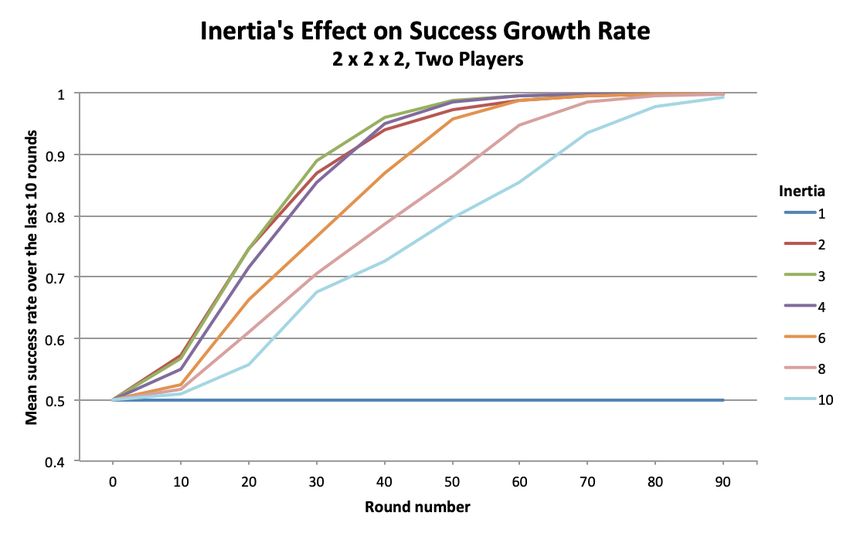
it is successful and each agent returns the ball drawn to the urn from which it was drawn and
adds a duplicate of that ball. If unsuccessful, each agent simply returns the ball drawn to the
urn from which it came. In this way successful dispositions are made more likely conditional
on the states that led to those actions.

                        nature                                                       action

                           0                                                            0
                                       sender             a         receiver
                                                          b
                           1                                                            1

                                        0     1                       a     b

                               Figure 1: a basic 2 × 2 × 2 signaling game

    Neither of the two signal types here begins with a meaning. If the agents are to be successful
in the long run, they must evolve signaling conventions where the sender communicates the cur-
rent state of nature by the signal she sends and the receiver interprets each signal appropriately
and produces the corresponding act. With unbiased nature, one can prove that the agents’
dispositions in the 2 × 2 × 2 signaling game under simple reinforcement learning will almost
certainly converge to a signaling system where each state of nature produces a signal that leads
to an action that matches the state.2
    More generally, however, n × n × n signaling games do not always converge to optimal
signaling systems on SR. For n = 3, about 0.09 of runs fail to converge to optimal signaling on
simulation. For n = 4, the failure rate is about 0.21. And for n = 8, the failure rate is about
0.59.3 When the game does not converge to an optimal signaling system, the players end up
in one of a number of sub-optimal pooling equilibria associated with various different success
rates.
    Lewis-Skyrms signaling games have been studied under a variety of different learning dy-
namics. One might punish agents by removing balls on unsuccessful plays, or add a mechanism
for forgetting past experience, or set a limit to the total number of balls of a given type in an
urn.4 Or one might consider different type of learning dynamics altogether.5
    When faced with the task of establishing a convention in the context of repeated plays of a
signaling game, human agents appear to use a low-rationality learning dynamics closely related
to win-stay/lose-shift (WSLS) (Cochran and Barrett, 2021). On WSLS the sender starts by
choosing a map from each possible state of nature to the signal she will send when she sees that
state. The receiver does the same, mapping each possible signal to the action he will perform
when he sees that signal. The dynamics does not require that the map from states to signals
or that the map from signals to actions is one-to-one or onto. The sender sends the signal that
the current state presently maps to, then the receiver sees the signal and performs the act that
the signal currently maps to. If the action matches the state, the agents are successful and they
keep their current maps in the next round. If the action does not match the state, the agents
are unsuccessful. In this case, the sender shifts strategies by mapping the state she just saw to
a new randomly-determined signal type and the receiver shifts strategies by mapping the signal
he just saw to a new randomly-determined action. There are no restrictions regarding how they
might shift strategies for the current state and signal (other than the new strategy must be
  2
    See Argiento et al. (2009) for the proof.
  3
    See Barrett (2006) for a discussion of these results and what they mean.
  4
    See Barrett and Zollman (2009) and Huttegger et al. (2014) for discussions of the effects of such modifications.
  5
    For examples see Huttegger et al. (2014) and Barrett et al. (2017).

                                                        2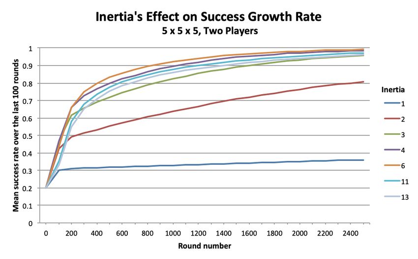
different from the old). The agents’ maps for states and signals they did not see on the current
play do not change.
     While the dispositions of agents using SR are determined by their full history of success
and failure, WSLS is very forgetful. Here the agents’ current strategy for each state and signal
type are determined by what happened the last time they saw the state or signal type. This
makes WSLS nimble and potentially quick at finding optimal signaling conventions. While
SR learners at best slowly converge to optimal signaling behavior and very often get stuck in
suboptimal partial pooling equilibria along the way, WSLS learners typically quickly converge
to optimal conventions—and when the game is relatively simple, they often converge to optimal
conventions in just a small number of plays.
     That said, there are two notable problems with WSLS. First, it is possible that both of the
agents will fail on a play of the game, both shift, both fail again, both shift again, etc. We will
call such systematic miscoordination the revolving-door problem. Second, WSLS is extremely
unstable in the context of noise or error. Agents might find a perfect signaling system, but if
the signal is ever mistransmitted, tampered with, or misread, this will generate an error causing
both agents to change their strategies. And since the new strategies will not be optimal, this will
typically lead to further errors and the unraveling of their hard-won conventions. The agents
then have to find their way back to an optimal signal system.6
     Human agents, however, use a variant of WSLS that avoids both of these problems. More
specifically, Cochran and Barrett (2021) show that the behavior of human subjects is well-
explained by the low-rationality dynamics win-stay/lose shift with inertia (WSLSwI). WSLSwI
is just like WSLS except that WSLSwI agents with inertia i shift to a new map from a state
to a signal (for senders) or from a signal to an act (for receivers) after i failures in a row for
the triggering signal or act.7 As we will see, WSLSwI is extremely well-suited to establishing
conventions quickly and reliably in the context of a broad array of signaling games. It is much
faster than SR and does not get stuck in suboptimal pooling equalibria. It is also much more
stable than WSLS in the context of noise, tampering, or error. And, for i ≥ 2 it avoids the
revolving-door problem.
     In the present paper, we investigate WSLSwI’s properties in detail. We start by showing
that WSLSwI learners converge to a signaling system with probability one for any m × m × m
Lewis signaling game and any inertia i except for the 2 ×2×2 game with i = 1. That said, there
may be evolutionary pressure for players to use inertia levels that are more successful sooner—
that is, more successful in the short and medium run. Specifically, we show that on simulation
a higher inertia level often allows for convergence to successful conventions faster than a lower
inertia level. This counter-intuitive phenomena is explained by the fact that inertia helps to
preserve the parts of a player’s total strategy that are optimal while the player seeks to fix by
trial-and-error those parts that are not yet optimal.8 We also discuss how the cognitive diversity
of agents may speed convergence to optimal conventions on this dynamics.
     While WSLSwI is a decidedly low-rational learning dynamics, one can make it more so-
phisticated by placing probabilistic constraints on the how agents choose a new strategy after
failing repeatedly.9 Cochran and Barrett (2021) found that human subjects do not shift strate-
gies randomly. Rather, they shift in a way that tends to preserve injective and/or surjective
strategy mappings. Since having such a mapping is a necessary global condition for having an
optimal signaling convention, such selective shifting might be considered a higher-rationality
   6
     While it is slow and subject to getting stuck in suboptimal pooling equilibrium, SR encounters neither of
these problems.
   7
     WSLS then is a special case of WSLSwI where i = 1.
   8
     For other discussions of the positive influence of some form of inertia in game play see Marden et al. (2009),
where they present a variant of fictitious play with inertia that always converges to a pure Nash equilibrium for
a certain class of game, and Laraki and Mertikopoulos (2015), where they investigate a variant of the replicator
dynamics with inertia.
   9
     This is also the idea behind Barrett et al. (2017).

                                                        3
version of WSLSwI.10 Here the focus is WSLSwI with random switching on repeated failure.
An investigation into higher-rationality versions of the dynamics is a natural next step.
We proceed as follows. The following section gives analytical proofs related to WSLSwI’s
convergence to a signaling system. Section 3 is broken into subsections which examine WSLSwI’s
behavior across a variety of parameter values: inertia level(s), number of states, and population
size. In section 4 we summarize our results and discuss a few outstanding questions for future
research.
2 Convergence in Win-Stay/Lose-Shift with Inertia
Because of the revolving-door problem WSLS (equivalently, WSLSwI with inertia i = 1 for both
players) does not always converge to a successful convention on 2 × 2 × 2 signaling games. We
now show that this case is the exception rather than the rule for WSLSwI. In particular, we
prove that in the two player 2 × 2 × 2 game in which at least one player does not have inertia
i = 1, WSLSwI players converge to a signaling system with probability 1 in the limit. More
generally, we show that in the two player m × m × m game with m > 2, WSLSwI players with
any inertia levels also converge to a successful convention with probability 1.
WSLSwI is a variant of Win-Stay/Lose-Shift. This means that it differs from the Win-
Stay/Lose-Randomize (WSLR) dynamics studied by Barrett and Zollman (2009).11 It is easy
to show that WSLR finds optimal signaling conventions with probability one since at every step
there is positive probability of it finding such conventions in a finite number of plays. But for
WSLSwI, the forced switch on failure (or a sequence of failures) makes the proof of convergence
more difficult. We break it into two smaller proofs. In each we specify an algorithm that
characterizes a positive probability path from an arbitrary state to a signaling system. Let
N = {N1 , N2 , . . . ., Nm }, S = {s1 , s2 , . . . ., sm }, and A = {a1 , a2 , . . . ., am } be the sets of states,
signals, and acts, respectively, and let aj be the appropriate act for state Nj . Let p1,t : N −→ S
and p2,t : S −→ A represent the sender’s12 and receiver’s stimulus response association at time
t. On each iteration of the game, both players obey their stimulus response association. That
is, if the sender witnesses state N ∈ N in round t, she will send signal p1,t (N ) to the receiver,
who will in turn perform act p2,t (p1,t (N )). Finally, let i1 and i2 represent the sender’s and
receiver’s inertia, respectively. Each time the players fail, they iterate their failure count for
that input by one before proceeding to the next round. If the sender’s failure count f1,t (N ) for
a particular state N reaches i1 , she shifts her mapping p1,t+1 (N ) to be a new signal. Likewise
for the receiver, whose failure count associated with signal s at time t is f2,t (s): if f2,t (s) = i2
at the end of round t, she will associate signal s with a new act in round t + 1. A player’s
failure count for a particular input (state for the sender, signal for the receiver) is reset to 0
when that player succeeds in a round on which that input was observed. We say that state Nj
is succeeding at time t if p2,t (p1,t (Nj )) = aj .
Proposition. In the two player m × m × m Lewis signaling game, WSLSwI players reach a
signaling system in the limit with probability 1 when either (or both) players have at least inertia
2.
Proof. We proceed by cases determined by inertia level and m.
CASE 1: Suppose that i1 ≥ 2 and i2 = 1. Consider the following algorithm for describing a
positive probability path to a successful signaling system.
10
One would not expect such higher-order selection in lower-cognition species.
11
WSLR is just like WSLS except that among the random possibilities the agent might choose not to modify
her strategy on failure.
12
We will use “1” throughout our notation to indicate a property of the sender (e.g. p1,t , inertia i1 , and f1,t ).
Similarly, we indicate the receiver with a “2”.
4• Step (1.1). If f1,t (N ) 6= i1 − 1 for every N ∈ N (that is, if no sender state-to-signal
mapping is just one failure away from reaching failure count i1 and thus switching), go
to step (1.2). Otherwise, repeat this step until f1,t (N ) 6= i1 − 1 for every N ∈ N . Each
iteration of this step takes a state of Nature with a failure count of i1 − 1 (i.e. the sender
is one failure away from shifting) and adjusts it to have inertia zero instead. Let Nj be
one such state of Nature with f1,t (Nj ) = i1 − 1. With positive probability, the following
happens:
– Period t: State Nj is selected by Nature. If the players succeed as a result, then
all players keep their mappings and f1,t+1 (Nj ) is reset to 0. If the players instead
fail then the sender’s failure count for state Nj reaches i1 , the sender readjusts her
mapping, and f1,t+1 (Nj ) is reset to 0.
• Step (1.2). If the sender’s map p1,t is bijective, proceed to step (1.3). Otherwise, repeat
this step until the sender’s mapping is bijective. Each iteration of this step takes two
states which map to the same signal and forces one to map to a different signal. Let Nj
and Nk be two such states that elicit the same signal from the sender: p1,t (Nj ) = p1,t (Nk ).
Since both states map to the same signal (call it s), at least one must be failing under
the current mappings. WLOG let Nj be failing i.e. p2,t (p1,t (Nj )) 6= aj . With positive
probability, the following happens:
– Period t: State Nj is selected by Nature, the sender sends s, and the receiver does
not choose act aj , resulting in a failure. Because f1,t (Nj ) 6= i1 − 1, the sender’s
mapping remains fixed. The sender’s failure count for state Nj is augmented by one:
p1,t+1 (Nj ) = p1,t (Nj ) + 1. The receiver adjusts her mapping such that p2,t+1 (s) = aj .
– Period t + 1: State Nk is selected by Nature, the sender sends s, and the receiver
chooses act aj , resulting in a failure. Because f1,t+1 (Nk ) 6= i1 − 1, the sender’s
mapping remains fixed. The sender’s failure count for state Nk is augmented by one.
The receiver adjusts her mapping such that p2,t+2 (s) = ak .
– Period t + 2: State Nk is selected by Nature, the sender sends s, and the receiver
chooses act ak , resulting in a success. The sender’s failure count for state Nk is reset
to zero: f1,t+3 (Nk ) = 0.
– Repeat these three steps until the sender’s failure count for Nj equals i1 . When that
happens, the sender changes her mapping so that Nj maps to an unused signal.
• Step (1.3). If players are in a signaling system, we are done. Otherwise, repeat this step
until the players are in a signaling system. Since players are not in a signaling system,
there must exist signal Nj such that p2,t (p1,t (Nj )) 6= aj . With positive probability, the
following happens:
– Period t: State Nj is selected by Nature, the sender sends p1,t (Nj ), and the re-
ceiver does not choose act aj , resulting in a failure. Because f1,t (Nj ) 6= i1 − 1,
the sender’s mapping remains fixed. The receiver adjusts her mapping such that
p2,t+1 (p1,t (Nj )) = aj . State Nj is now succeeding.
CASE 2: Suppose that i2 ≥ 2. Consider the following algorithm for constructing a positive
probability path from players’ current dispositions to a successful signaling system.
• Step (2.1). If at least one state is succeeding under the current mappings at time t,
go to step (2.2). Let aj ∈ A be an act such that there exists s ∈ S with p2,t (s) = aj .
With positive probability, the sender observes Nj for min[i1 − f1,t (Nj ), i2 − f2,t (p1,t (Nj ))]
5consecutive periods (failures). At this point either the sender or the receiver (or both)
will adjust their mapping. If it’s the sender (or both), she shifts so that p1,t+1 (Nj ) = s.
If it’s the receiver, he shifts so that p2,t+1 (p1,t (Nj )) = aj . Either way, state Nj is now
succeeding.
• Step (2.2). If p1,t is bijective, go to step (2.3). Otherwise, repeat this step until a
bijection is formed for the sender. Since p1,t is not bijective, there must exist two states
Nj and Nk such that p1,t (Nj ) = p1,t (Nk ). Since both states map to the same signal s,
at least one of these states must be failing. WLOG, let Nj be failing. With positive
probability, the following happens:
– Subcase 2.2.1) State Nk is succeeding. Nature repeatedly alternates between states
Nk and Nj for i1 − f1,t (Nj ) plays. Each time Nk is selected, the receiver’s failure
count for signal s is reset to 0. Each time Nj is selected, the failure count for Nj
increases by 1. After i1 − f1,t (Nj ) occurrences of Nj (all failures) the sender updates
her stimulus response association so that Nj maps to an unused signal. State Nk is
still succeeding.
– Subcase 2.2.2) State Nk is failing (in addition to Nj ). This case is only possible when
m > 2. Nature chooses Nk for i1 − f1,t (Nk ) consecutive rounds. The receiver may
change the act she associates with s = p1 (Nk ) during this time. If the latter happens,
the receiver now maps signal s to a new act that is not ak (which is possible because
there are at least three acts in this subcase). If the receiver switches this mapping
again before the end of the i1 − f1,t (Nk ) occurrences of Nk , she resumes her original
failing mapping. The receiver toggles between these two failing mappings for the
duration of these i1 − f1,t (Nk ) occurrences of Nk . Each of these plays is a failure,
so the sender adjusts her stimulus response association to map state Nk to a new
unused signal.
• Step (2.3). If players are in a signaling system, then we are done. Otherwise, repeat
this step until players are in a signaling system. Each iteration of this step increases the
number of succeeding states by 1. The sender’s mapping is now in a bijection and at
least one state is succeeding. All that remains is to jiggle the receiver’s mapping into a
complementary bijection. Let Nj be a succeeding state. Let Nk be a failing state which
currently maps to state s. With positive probability, the following happens:
– Nature repeatedly alternates between state Nj and Nk . Players always succeed on
the former and fail on the latter (increasing the failure counts for state Nk and signal
s. After i1 − f1,t (Nk ) occurrences (failures) of Nk , the sender must map state Nk to a
different signal. She maps it to p1,t (Nj ), the same signal used to represent succeeding
state Nj .
– Nature continues to alternate between Nj and Nk . Now whenever Nk occurs, act
aj is chosen and players fail. This augments f1 (Nk ) by 1 and f2 (p2 (Nk )) by 1. In
the subsequent round, Nj is chosen and players succeed, resetting f2 (p2 (Nk )) to 0.
Since the receiver’s inertia is at least 2, this prevents the receiver from switching
their mapping which facilitates state Nj ’s success. After i1 more occurrences of Nk
(all failures), the sender must map Nk to a new signal. She maps it back to her old
signal s.
– This process repeats: Nature waffles back and forth between state Nj and Nk , the
sender maps Nk back and forth between s and p1,t (Nj ), and the receiver’s failure
count for s grows on any round in which Nk is the state and the sender chooses s.
Eventually the receiver’s failure count for s equals i2 and she must switch. She does
so by mapping signal s to act ak . State Nk is now succeeding.
6Case 1 and 2 give a positive probability path to a signaling system from any player state.
One of these must be the longest path (of length n) in terms of number of plays required to
reach it, and one of these must be the least probable (with probability e). Thus, the probability
of not being absorbed into a signaling system after n plays from an arbitrary player state is at
most 1 − e. The probability of not being absorbed after z ∗ n plays is then (1 − e)z . The limit
of this expression as z → ∞ is 0. Thus, the probability of being absorbed in the long run is
1 and it was sufficient to show that there exists a positive probability path from any arbitrary
state to an absorbing signaling system.
We now show the same thing for larger games and players with inertia exactly 1 (recall that
players are not guaranteed to converge to perfect signaling for the 2 × 2 × 2 game with inertia
1 for both players).
Proposition. In the two player m × m × m Lewis signaling game with m > 2 and inertia level
1 for both agents, players converge to a signaling system in the limit with probability 1.
Proof.
• Step (1). If there exists s ∈ S such that the sender maps all states to s, go to step (2).
Otherwise, repeat this step until all states map to the same signal. Choose an arbitrary
signal s. Let N be a state which does not map to s. If N is failing, then, with positive
probability, N is chosen and the sender adjusts her mapping so that p1,t (N ) = s. If N is
succeeding, then the following happens with positive probability:
– Period t: Let N 0 be a state that is not succeeding (which must exist if players are
outside a signaling system). On this play, N 0 is chosen, players fail, and the sender
adjusts her mapping so that p1,t+1 (N 0 ) = p1,t (N ).
– Period t + 1: State N 0 is chosen again. Since N 0 now maps to the same signal as
N , a succeeding state, this play must fail. The sender shifts back to her previous
mapping: p1,t+2 (N 0 ) = p1,t (N 0 ). The receiver also switches, meaning N is no longer
a succeeding state.
– Period t + 2: State N is chosen, players fail, and the sender adjusts her mapping:
p1,t+3 (N ) = s.
• Step (2). Let s be the signal to which the sender maps all states. If the receiver’s
mapping p2,t on the set S − {s} is an injection, go to step (3). Otherwise, repeat this step
until it is. Since the receiver’s mapping from signals (excluding s) to acts is not bijective,
there must exist two signals sj 6= s and sk 6= s which map to the same act al . With
positive probability, the following happens:
– Period t: Let N be a state such that N 6= Nl and N is not succeeding. (Exactly one
state is succeeding because they all map to s. Since there are at least three states,
there must be at least one which is not the succeeding state and not Nl .) State N is
chosen. Players fail and the sender adjusts her mapping so that p1,t+1 (N ) = sj .
– Period t + 1: State N is chosen again. The sender sends sj . The receiver sees this
and chooses act al . Since N 6= Nl , this fails. The sender switches back so that she
maps N to s. The receiver switches so that sj maps to an unused act.
• Step (3). If there are exactly three states currently mapping to s, go to step (4). Oth-
erwise, repeat this step until there are. Again, let s be the signal to which all states
currently map. There is also exactly one act al such that no signal in S − {s} maps to al ,
since |S − {s}| = |A| − 1 and the receiver’s mapping on S − {s} is injective. With positive
probability, the following happens:
7– Period t: Let Nj be a failing state such that Nj 6= Nl . On this play, Nj is chosen
and players fail. Since p2,t is injective on S − {s}, there must exist exactly one
signal s∗ ∈ S − {s} such that p2,t (s∗ ) = aj . The sender adjusts her mapping so that
p1,t+1 (Nj ) = s∗ . The receiver adjusts her map so that s maps to some new act. State
Nj is now succeeding (Nj maps to s∗ which maps to aj ) and there is one fewer state
that maps to s.
• Step (4). Executing this step once will put players in a signaling system. Similar to step
(3), let s be the signal to which exactly three states currently map and al be the act such
that no signal in S − {s} maps to al . There are exactly three states currently mapping
to s, denote Nj and Nk as the two non-Nl states which map to s. Since they map to
the same signal, at least one of Nj and Nk must be failing. WLOG, say it is Nj . With
positive probability the following happens:
– Period t: On this play, Nj is chosen and players fail. Since p2,t is a bijection, there
must exist exactly one signal s∗ ∈ S − {s} such that p2,t (s∗ ) = aj . The sender
adjusts her mapping so that p1,t+1 (Nj ) = s∗ . The receiver adjusts her map so that
p2,t+1 (s) = aj . State Nj is now succeeding and there are exactly two states that map
to s. All others states are succeeding.
– Period t + 1: On this play, Nk is chosen, signal s is sent, act aj is chosen, and players
fail. By construction there must exist exactly one signal s∗ ∈ S − {s} such that
p2,t+1 (s∗ ) = ak . The sender adjusts her mapping so that p1,t+2 (Nk ) = s∗ . The
receiver adjusts her map so that p2,t+2 (s) = al . State Nk is now succeeding. Also,
since p2,t+2 (p1,t+2 (Nl )) = al , state Nl is also now succeeding. Players are now in a
signaling system.
Thus, as in the last proof, there exists a positive probability path from any state to a
signaling system, so players must enter a signaling system eventually with probability 1.
3 Simulation results
The upshot of these results is that agents will reach a signaling system with probability 1 in all
but the 2 × 2 × 2 game with inertia i = 1 for both players. In this section we consider simulated
agents playing a repeated m × m × m signaling game for various inertia i, game size m, and
population size. This provides a sense of what matters for the rate of convergence of WSLSwI.13
3.1 The 2 × 2 × 2 signaling game under WSLSwI
Let’s start simple. Suppose two WSLSwI players, a sender and receiver, engage in a repeated
2 × 2 × 2 signaling game. Suppose further that the two players have the same inertia level i.
We will first consider how the inertia i affects the speed at which agents approach a signaling
system. In figure 2 graph measures the mean success rate over every 10 round interval for
simulated agents with i = 1 (in dark blue), i = 2 (red), etc. Some inertia levels are omitted for
the sake of visibility.
First, concerning the horizontal line at a success rate of 0.5, players with i = 1 do not
in aggregate approach a successful convention. This is because of the revolving door problem.
Consider WSLSwI in the 2×2×2 game as a Markov chain. There are 16 distinct mapping states
in which players might start. Two of these are signaling systems, granting payoff 1. The other
fourteen start and remain in one of three ergodic sets, through which they wander forever,
13
All simulations were programmed in Eclipse, a JAVA based IDE. Each inertia level was run for 105 iterations.
8Figure 2: Success rate as a function of (equal) inertia for two players in a repeated 2 × 2 × 2
signaling game.
never achieving optimal conventions. The first of these is illustrated in figure 3; it contains
six mapping states and has average payoff 31 (calculated from the stable state probabilities).
The other two sets each contain four mapping states and have expected payoff 12 in each of
these states. The expected payoff of a player pair starting with random dispositions is then
2 6 1 4 1 4 1
16 · 1 + 16 · 3 + 16 · 2 + 16 · 2 = 0.5. This matches our simulations where the agents’ mean overall
success rate hovers near 0.5.
In contrast, the other tested inertia levels rapidly approach perfect signaling both individu-
ally and in aggregate on simulation. And the convergence is fast. All are nearly optimal after
just 90 rounds. While all are fast, some are faster than others.14 Significantly, speed is not
monotonic in inertia i: there exists a fastest i strictly between 2 and 10. On quick inspection,
the fastest inertia is near i = 3 (though i = 2 has a small edge in the early game).15 This
non-monotonicity in speed can be understood through a trade-off that goes hand-in-hand with
increasing inertia. One side of this trade-off is immediate: having too much inertia can be bad.
Players with a very high inertia seldom change their dispositions even when they have good
reason to do so. As an extreme example, agents with i = 91 would have never changed their
starting dispositions in the first 90 rounds shown in figure 2 (though, as proven in the last
section, they will eventually reach a signaling system in the long run).
The reason that more inertia can hasten evolution to optimal conventions is more subtle.
Suppose players’ stimulus response associations are represented by figure 4 on the left. This is
not a signaling system, but one of the states of nature (state 1) is succeeding as a result of the
players’ current mappings. If players could preserve the state 1 mappings (i.e. nature 1 maps
14
We are concerned here with speed in the early and medium run that might give the agent an evolutionary
advantage. We do not split hairs between already-successful players in the late-game.
15
The difference between the lines representing inertia levels 2, 3, and 4 is quite small, perhaps to the point
where the non-monotonicity in speed is difficult to verify via a cursory inspection. The difference in speed is
more dramatic in larger games, as we will see.
9Sender’s signal Receiver’s act
Nature 1 Act 1
Nature 2 Act 2
Sender’s signal Receiver’s act Sender’s signal Receiver’s act
Nature 1 Act 1 Nature 1 Act 1
Nature 2 Act 2 Nature 2 Act 2
Sender’s signal Receiver’s act
Nature 1 Act 1
Nature 2 Act 2
Sender’s signal Receiver’s act Sender’s signal Receiver’s act
Nature 1 Act 1 Nature 1 Act 1
Nature 2 Act 2 Nature 2 Act 2
Figure 3: Flow chart illustrating a revolving door problem between two players utilizing Win-
Stay/Lose-Randomize learning. Bold arrows represent possible transitions between player
states. Both players repeatedly miscoordinate and adjust their mappings but never reach a
signaling system. They would be able to reach a stable convention if occasionally only one
player adjusted her mapping; this is possible in Win-Stay/Lose-Randomize with Inertia.
Sender’s signal Receiver’s act Sender’s signal Receiver’s act
Nature 1 Act 1 i=1 Nature 1 Act 1
Nature 2 Act 2 Nature 2 Act 2
Figure 4: Illustration of how low inertia may jeopardize player mappings corresponding to
successful states.
to signal 2 which maps to act 1) and simply fiddle with the others until state 2 also succeeds,
this seems like a speedy way to reach a signaling system. Successful mappings for individual
states can be difficult to maintain for low inertia players, though, especially if the sender’s map
is not bijective. If nature 2 is selected and i = 1 in figure 4, then players fail and readjust their
mappings for state 2 and signal 2, destroying the successful mapping in the process.
But consider what happens in this scenario when players have an inertia of i = 4. Nature’s
selection of state 2 no longer immediately alters the players’ successful mappings for state 1.
Instead, agents’ failure counts for the appropriate stimuli simply increase by 1. It would take
four consecutive realizations of state 2 for players to lose the fruitful state 1 mappings. What
happens if these four occurrences of state 2 are interrupted by just one instance of state 1?
Players will succeed on that play, and this resets the receiver’s failure count for its signal 2
mapping to 0. Importantly, though, the sender’s failure count for its state 2 mapping is not
reset. After the 4th (not necessarily consecutive) occurrence of state 2, the sender’s failure
count for this state is 4, forcing her to switch that mapping (while the receiver keeps hers). The
sender’s mapping is now a bijection and all that remains is for the receiver to change her signal
1 mapping16 . The higher the agents’ inertia i, the less likely i consecutive occurrences of the
failing state of nature will transpire, preserving the receiver’s successful mapping.
To summarize, the trade-off for high inertia learning works as follows. An efficient way for
players to reach a signaling system is to secure a successful mapping for one state and then
the other. Once one successful mapping for a state is secured, the sender’s map for this state
is stable but the receiver’s may not be. Having higher inertia strengthens the stability of the
16
This will take a few more plays, and the sender will actually have to revert to her old state 2 mapping
temporarily. Barring four sequential occurrences of state 2, though, players will reach a successful convention.
10receiver’s advantageous mapping, allowing players to hold the mappings for the successful state
steady while those of the other state are being constructed via trial and error. On the other
hand, the added stability benefit from an uptick in inertia comes with the obvious cost of players
tuning their dispositions less often in response to failure. A healthy dose of inertia promotes
speed—but too much yields sluggishness. Hence, there exists an inertia level above 1 which
maximizes players’ speed in approaching a signaling system. This is true in the 2 × 2 × 2 game
and in the larger games we investigate in the next subsection.
3.2 Larger games
In the simple 2 × 2 × 2 game, the speeds for i = 2 and i = 3 were neck-and-neck and the
non-monotonicity of speed as a function of inertia is difficult to see. It is more conspicuous for
larger games. Figures 5 and 6 plot the average success rate growth at different inertias for the
two player 5×5×5 and 10×10×10 games, respectively. Note that tick marks on the x-axis now
represent 100s of plays as these are much more complicated games, and we measure players’
average success every 100 plays. In contrast, simple reinforcement learning is much slower than
WSLSwI at many inertia levels greater than 1. SR also often encounters suboptimal pooling
equilibria that prevent agents from converging to optimal conventions on the 5 × 5 × 5 game,
and it is much slower yet and nearly always fails to converge to optimal signaling on simulation
in the 10 × 10 × 10 game.
Figure 5: Success rate as a function of (equal) inertia for two players in a repeated 5 × 5 × 5
signaling game.
In accord with the analytic results in the previous section, inertia i = 1 does appear to be
slowly evolving toward a successful convention in the 5 × 5 × 5 game as there is no revolving
door to hold it back. WSLSwI with inertia i = 2 does much better and an inertia of i = 3 does
much better still. These gains in speed for larger inertia illustrate the, now more pronounced,
trade-off benefit discussed in the last section. Namely, high inertia allows players to maintain
successful mappings for individual states prior to reaching a signaling system. The stability of
11Figure 6: Success rate as a function of (equal) inertia for two players in a repeated 10 × 10 × 10
signaling game.
these mappings increases monotonically with inertia, but the returns are diminishing. In the
5×5×5 game, inertia i > 6 becomes more of a hindrance than a blessing, as successful mappings
are already relatively stable but agents are sitting on their failing mappings for longer periods.
Similarly in the 10 × 10 × 10 game where extra speed increases monotonically with speed to
inertia i = 8 then declines.
Note that while the non-monotonicity of speed as a function of inertia is universal across
all of our game sizes, the inertia level that maximizes growth rate is not. When m = 2, the
optimal i for speed is about 3. For m = 5 it is 6. For m = 10, it is 8. There are at least two
influencing factors here. First, larger games take longer to master. Even after 6,000 plays, the
inertia 8, WSLSwI 10 × 10 × 10 players have only just broken an average payoff of 0.9.17 During
this time agents are gradually evolving their dispositions to be more successful for more states.
Successful state mappings of the receiver can be broken by i consecutive occurrences of a failing
state without interruption by the relevant successful one, as detailed in the previous subsection.
While an inertia of, say, i = 4, may seem safe because it is unlikely that the failing state will
be selected this many times consecutively, it may not be. Larger games require more periods of
experimentation before a convention is reached, and there is plenty of time for the failing state
to be chosen repeatedly and for a good mapping to be abandoned. Second, with larger games
comes the possibility that the sender may map three, four, or more states to the same signal s.
Suppose one of these states is succeeding. All of the other states which the sender maps to s
must then be failing, and i consecutive occurrences of any of these unsuccessful states will force
a switch from the receiver. Hence, in larger games it pays to have more patience for failure.
Note that in the 10 × 10 × 10 game, while it may not appear from the graphs that the i = 1
and i = 2 inertia players are experiencing any growth in average success rate, they are—it is
17
That said, this is infinitely better than SR does in this large a game, as it typically just gets stuck in
suboptimal pooling equilibria.
12just too small to observe the growth at this scale. That said, it is extremely difficult for these
low inertia players to evolve a signaling system. Any successful state mappings are typically
fleeting, as very few failures are needed to convince the receiver to abandon her previous map.
What little growth there is can be traced to the trickle of sender-receiver pairs (out of the
100,000 pairs corresponding to each run) in every round who were lucky enough to stumble
their way into a signaling system.
In summary, WSLSwI has significant advantages over both simple reinforcement learning SR
and WSLS. WSLSwI is much faster than SR. It consequently explains how human subjects are
often able to converge to a set of optimal signaling conventions very quickly.18 Further, unlike
SR, WSLSwI explains how agents may fully converge to optimal conventions in a finite time.
And, also unlike SR, WSLSwI is not prone to getting stuck in suboptimal pooling equilibria in
signaling games. Indeed, as we have shown, WSLSwI converges to perfect signaling for i ≥ 2.
The i = 1 version of WSLSwI (WSLS), is the only case that encounters the revolving door
problem. This case is also the least stable version of WSLSwI at equilibrium as a single error
can lead to a chain of mistakes that unravel the agents’ hard-won conventions. Finally, as we
have just seen, increasing the inertia can make WSLSwI faster in establishing conventions as a
result of the corresponding increase in the stability of the dynamics.
For all its virtues, WSLSwI does not do as well as SR in signaling games where there are
fewer signals than states or acts. In a 3 × 2 × 3 signaling game, a WSLSwI learner will keep
shifting strategies forever in an effort to get a bijection between states and signals and signals
and acts. In contrast, an SR learner will learn to play a strategy that succeeds an optimal 2/3
of the time on this game.19 This is only a problem, however, if the agents fail to have sufficient
signals to represent the states of nature that are salient to successful action and are unable to
produce new signals.
3.3 Differing inertia levels between sender and receiver
The simulations of the previous subsections featured senders and receivers with equal inertia.
This need not be the case, and given what we have seen so far regarding the subtlety of the
relationship between speed and inertia, one might naturally wonder whether there might be
a benefit to an inertial discrepancy between agents. As a first guess, one might predict that
heterogeneity in inertia between sender and receiver simply leads to a success rate that falls
between the homogeneous inertia speeds. That is, the average speed with which a sender of
inertia 5 and a receiver of inertia 6 approach a signaling system is between the speed of two
players with inertia 5 and two players with inertia 6. But this is not typically the case.
Consider figure 7, which displays the progress of players with the following (sender, receiver)
inertia level pairs: (5, 7); (7, 5); (5, 5); (6, 6); (7, 7). We see that, in the short and medium run,
(5, 7) leads the pack, followed by (7, 5). Both of them perform better than their pure inertia
(5, 5) and (7, 7) counterparts20 . The mixed inertia curves even outpace the (6, 6) curve, which
maximized speed over all tested homogeneous inertia levels for m = 5.
This phenomenon is not unique to these inertia values. In general, heterogeneous inertia
levels usually perform better than their homogeneous counterparts on simulation. Further, for
a pair of different inertia values x and y, with x < y, we typically saw (x, y) grow faster than
(y, x). That is, agents tend to do better when the sender has less inertia than the receiver rather
than the other way around. Given the evidence, we believe that there is a speed benefit to the
sender having more inertia than the receiver and a speed benefit to the receiver having more
inertia than the sender, but the latter effect is stronger. We can make some rough guesses as
to why we see this collection of phenomena.
18
See Cochran and Barrett (2021).
19
See Cochran and Barrett (2021) for a discussion of the problems human learners have with this game.
20
The curve for (5, 5) inertia is difficult to see; it is underneath the arcs for (6, 6) and (7, 7)
13Figure 7: Success rate as a function of (not necessarily equal) inertia for two players in a
repeated 5 × 5 × 5 signaling game.
Suppose the sender’s and receiver’s dispositions in a 3 × 3 × 3 game are partially represented
in figure 8 on the left. Currently, state 2 is succeeding and it would be to players’ benefit to
preserve the mappings facilitating this (i.e. state 2 maps to signal 2 which maps to act 2).
Consider how this might be jeopardized. The sender’s part of this map is stable (for now):
whenever state 2 is realized, they succeed. However, the receiver’s map from signal 2 to act
2 may be endangered by multiple consecutive occurrences of state 3, each of which results in
failure and augments the receiver’s failure count for state 2 by one. A higher inertia level for
the receiver increases her resilience in the face of these failures. In addition, lower sender inertia
will result in the sender adjusting her failing state 3 map sooner; it then no longer threatens the
players’ successful state 2 mapping. Thus, low sender and high receiver inertia may promote
agents’ success growth rate.
Sender’s signal Receiver’s act Sender’s signal Receiver’s act
Nature 1 Act 1 Nature 1 Act 1
Nature 2 Act 2 Nature 2 Act 2
Nature 3 Act 3 Nature 3 Act 3
Figure 8: Two partial sender and receiver mappings in a 3 × 3 × 3 game.
The benefits of the sender having higher inertia than the receiver are less clear, but here is
our best guess at what drives the phenomena. Consider the partial sender and receiver mapping
on the right in figure 8. Currently, state 1 is failing. Suppose that the players have equal inertia
14level i and their current failure count for the displayed mappings is 0. After i rounds of failure
on state 1, both agents will switch their mapping. While there is no way to say whether their
new mappings will be profitable, one might estimate each of their new mappings have something
like a 13 chance of being successful since m = 3. Suppose that the sender has an inertia of, say,
4, and the receiver’s is 3 for the same initial mapping on the right of the figure. After 3 failures
on state 1, the receiver switches and has a 12 (slightly better than 13 ) chance of mapping signal
1 to act 1, thus making state 1 a successful state and resetting the sender’s state 1 failure count
to 0 on that state’s next occurrence. If she instead maps signal 1 to act 3, the sender still has
an approximately 13 chance to make a successful mapping on the next play. Thus, less inertia
for the receiver may give players a slight edge in their search for success. Of course, players
in the right-hand mapping may not start with the same failure counts. However, higher on
average inertia for the sender means that the receiver switches before the sender on average, so
the effect described in this paragraph should still often hold.
It is important not to miss the central point here in the details. Our simulations repeat-
edly suggest that differences in inertia help to speed convergence to optimality in two-player
signaling games under WSLSwI. This represents a concrete virtue for a particular variety of cog-
nitive diversity. Other things being equal, agents with different levels of patience may benefit
significantly from those differences in the establishment of convention.
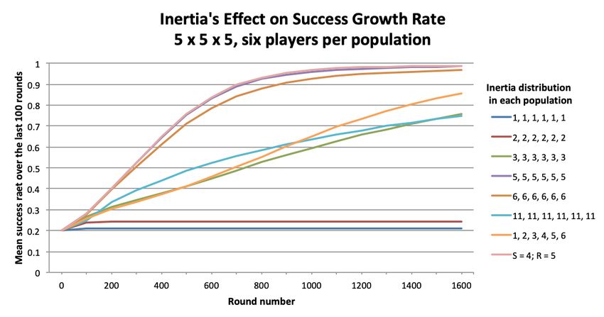
3.4 Population games
The human subjects in the experiments described by Cochran and Barrett (2021) were not
paired with a single partner for every play of the signaling game. Rather, six subjects were
assigned to the sender group and six to the receiver group. Then, on each play of the game, a
random sender was paired with a random receiver.21 On this sort of population game, one is
considering how conventions might evolve for an entire community as agents learn from their
random interactions.
Consider n simulated senders and n simulated receivers randomly matched in each round to
play an m × m × m signaling game. The graph for players’ progress in the 5 × 5 × 5 game with
populations of size 6 is displayed in figure 9 as an example. Every 100 plays, the average success
of the group over those 100 plays is measured and plotted. Different color curves represent the
different inertia distributions depicted in the key and present in both populations (with the
exception of the last series, which indicates that all senders had inertia 4 and all receivers had
inertia 5).
There are a number of robust phenomena in the population games we considered. First,
agents do converge to a signaling system under WSLSwI.22 Second, when all players have the
same inertia, we observe the same non-monotonicity in speed as a function of inertia that
occurred in the two-player simulations. Each specified population and game size pair has an
optimal inertia greater than 1 that maximizes its convergence speed. But this optimal inertia
for the population games was often different from the two player games. In fact, sometimes it
was smaller. For instance, in the 5 × 5 × 5 game with two players, we observed that the average
speed maximizing inertia level was i = 6. For the population game with 6 players each, though,
it was i = 5.23 Third, low inertia learning is yet more ineffective in the context of a population
game. For instance, while the growth of inertia i = 1 and i = 2 players is pronounced enough
to be seen in figure 5, the average progress of our population game players with these inertias
cannot be detected in figure 9 (though it is really just growing very slowly). This agrees with the
21
In this regard, the experiments described in Cochran and Barrett (2021) follow the protocol established in
Bruner et al. (2018).
22
This is for the same reason as in the two-player case. Indeed, the proof of the earlier theorem can be easily
extended to population games.
23
It is not at all clear to us why this should be the case. Figuring this out will require further careful
investigation.
15Figure 9: Success rate as a function of (not necessarily equal) inertia for populations of size six
in a repeated 5 × 5 × 5 signaling game.
intuition that when functioning dispositions are difficult to maintain, as they are when inertia
is low, adding more players who must each learn to agree on their mappings does not accelerate
progress. Finally, for the few population games in which we tried heterogeneous inertia between
senders and receivers, we observe that such differences often slightly boosts players’ speed to
a signaling system, mirroring our two player findings. For instance, in figure 9, players with
i1 = 4 and i2 = 5 perform better on average than in runs where all players had inertia 4 or all
had inertia 5. Here cognitive diversity serves the interests of the entire community.
4 Discussion
Win-Stay/Lose-Shift with Inertia WSLSwI is a low-rationality dynamics that is singularly well-
suited to establishing conventions in Lewis-Skyrms signaling games. Given its efficacy, it is
understandable that human subjects tend to use it for just this purpose as shown by Cochran
and Barrett (2021). But it remains a notable adaptation as it is unlikely that people realize
the virtues of the dynamics (or even that they use it) in just those situations where it works so
well.
Not only does WSLSwI always converge to a signaling system for inertia greater than 1, but
increased inertia contributes to the stability of the dynamics and often, remarkably, also speeds
convergence to an optimal set of conventions. As reported in Cochran and Barrett (2021),
human subjects also take advantage of this fact. Again, it is unlikely that they do so knowing
what they are doing or why it works. Finally, we have considered how cognitive diversity may
serve the interests of the entire community by speeding convergence to optimal conventions
under the present dynamics.
In addition to the open questions we have discussed along the way, there are a number of
issues concerning the behavior of WSLSwI yet to explore. While some combinations of inertia
levels one might assign to players in a population game underperform (such as when population
members have inertia levels 1, 2, 3, 4, 5, and 6 as in figure 9) other combinations excel. One
might seek to determine what combinations of cognitive diversity are optimal in a particular
16population game.
We have supposed that an agent’s inertia is constant over time. The human subjects studied
in Cochran and Barrett (2021), however, tend to exhibit increased inertia the longer they play
a game. Allowing inertia to evolve has manifest virtues. If agents have established an optimal
convention, then it makes sense to lock it in with higher inertias. One might also consider
the possible virtues of an agent tuning her inertia conditional on the behavior of other agents.
Given the virtues of cognitive diversity exhibited in the simulations considered here, one might
also consider what happens when agents draw their inertia levels in each round of play from a
distribution. And, of course, that distribution might itself evolve over time.
There is one last feature of WSLSwI and human behavior to discuss. Throughout this
paper we supposed that WSLSwI agents shift randomly on repeated failure. This is in keeping
with the thought of WSLSwI as a low-rationality dynamics. That said, the human subjects
in Cochran and Barrett (2021) did not always shift randomly. Rather, many of their shifts
reflected higher-order considerations. More specifically, the human agents tended to preserve
the injectivity and surjectivity of the maps from states to signals and signals to acts necessary
for optimal signaling. In this regard WSLSwI serves as a general framework for trial and error
learning. By stipulating when and how shifts occur, WSLSwI might be transformed from a
generic low-rationality dynamics to a higher-rationality dynamics, perhaps one especially well-
suited to a particular task. Of course, one might also allow an agent’s strategy for when and
how to shift on failure to itself evolve over time and from one context to another.
There is a rich collection of variants of WSLSwI to explore. The sort of learning exhibited
by human subjects playing Lewis-Skyrms signaling games is a special case.
Bibliography
Argiento, Raffaele, Robin Pemantle, Brian Skyrms, and Stanislav Volkov (2009). “Learning to
Signal: Analysis of a Micro-level Reinforcement Model.” Social Dynamics, 225–249.
Barrett, Jeffrey (2006). “Numerical Simulations of the Lewis Signaling Game: Learning Strate-
gies, Pooling Equilibria, and the Evolution of Grammar.” UC Irvine: Institute for Mathe-
matical Behavioral Sciences Technical Report.
Barrett, Jeffrey and Kevin Zollman (2009). “The role of forgetting in the evolution and learning
of language.” Journal of Experimental and Theoretical Artificial Intelligence, 293–309.
Barrett, Jeffrey A., Calvin T. Cochran, Simon Huttegger, and Naoki Fujiwara (2017). “Hybrid
learning in signalling games.” Journal of Experimental and Theoretical Artificial Intelligence,
29 (5), 1119–1127.
Bruner, Justin, Cailin O’Connor, Hannah Rubin, and Simon M. Huttegger (2018). “David
Lewis in the lab: experimental results on the emergence of meaning.” Synthese, 195 (2),
603–621.
Cochran, Calvin and Jeffrey Barrett (2021). “How signaling conventions are established.”
Synthese, https://doi.org/10.1007/s11229–020–02982–9.
Erev, I. and A.Ẽ. Roth (1998). “Predicting how people play games: reinforcement learning
in experimental games with unique, mixed strategy equilibria.” American Economic Review,
88, 848–881.
Herrnstein, R.J̃. (1970). “On the law of effect.” Journal of the Experimental Analysis of
Behavior, 13, 243–266.
17Huttegger, S., B. Skyrms, P. Tarres, and E. Wagner (2014). “Some dynamics of signaling
games.” Proceedings of the National Academy of Sciences, 111 (Supplement 3), 10873–10880.
Laraki, Rida and Panayotis Mertikopoulos (2015). “Inertial Game Dynamics and Applica-
tions to Constrained Optimization.” SIAM Journal on Control and Optimization, 53 (5),
3141–3170.
Lewis, David Kellog (1969). Convention: a philosophical study. Harvard University Press.
Marden, Jason R., Guerdal Arslan, and Jeff S. Shamma (2009). “Joint Strategy Fictitious
Play With Inertia for Potential Games.” IEEE Transactions on Automatic Control, 54 (2),
208–220.
Skyrms, Brian (2010). Signals: Evolution, Learning, and Information. Oxford University Press.
18You can also read