RangeRCNN: Towards Fast and Accurate 3D Object Detection with Range Image Representation
←
→
Page content transcription
If your browser does not render page correctly, please read the page content below
RangeRCNN: Towards Fast and Accurate 3D Object Detection
                                                            with Range Image Representation
                                                             Zhidong Liang1 , Ming Zhang1 , Zehan Zhang1 , Xian Zhao1 , and Shiliang Pu1

                                            Abstract— We present RangeRCNN, a novel and effective
                                         3D object detection framework based on the range image
                                         representation. Most existing methods are voxel-based or point-                                      (a) Range Image
                                         based. Though several optimizations have been introduced to
                                         ease the sparsity issue and speed up the running time, the two
arXiv:2009.00206v2 [cs.CV] 23 Mar 2021

                                         representations are still computationally inefficient. Compared
                                         to them, the range image representation is dense and compact
                                         which can exploit powerful 2D convolution. Even so, the range
                                         image is not preferred in 3D object detection due to scale
                                         variation and occlusion. In this paper, we utilize the dilated
                                         residual block (DRB) to better adapt different object scales                       (b) Voxel                                 (c) Point
                                         and obtain a more flexible receptive field. Considering scale
                                         variation and occlusion, we propose the RV-PV-BEV (range               Fig. 1.     Different representations of point clouds. (a) Range image
                                         view-point view-bird’s eye view) module to transfer features           representation (dense). Use 2D convolution to extract features. (b) 3D Voxel
                                         from RV to BEV. The anchor is defined in BEV which                     representation (sparse). Use 3D convolution to extract features. (c) Point
                                         avoids scale variation and occlusion. Neither RV nor BEV can           representation (sparse). Use point-based convolution to extract features.
                                         provide enough information for height estimation; therefore, we
                                         propose a two-stage RCNN for better 3D detection performance.
                                         The aforementioned point view not only serves as a bridge
                                         from RV to BEV but also provides pointwise features for                which limits its performance. The point-based representation
                                         RCNN. Experiments show that RangeRCNN achieves state-of-               retains more information than the voxel-based methods.
                                         the-art performance on the KITTI dataset and the Waymo                 However, the point-based methods are generally inefficient
                                         Open dataset, and provides more possibilities for real-time 3D
                                                                                                                when the number of points is large. Downsampling points
                                         object detection. We further introduce and discuss the data
                                         augmentation strategy for the range image based method, which          can reduce the computation cost but simultaneously degrades
                                         will be very valuable for future research on range image.              the localization accuracy. In summary, neither of the two
                                                                                                                representations can retain all original information for feature
                                                              I. INTRODUCTION                                   extraction while being computationally efficient.
                                            In recent years, 3D object detection has attracted increas-            Although we mostly regard the point cloud as the raw data
                                         ing attention in many fields. The well-studied 2D object               format, the range image is the native representation of the
                                         detection can only determine the object position in the 2D             rotating LIDAR sensor (e.g. Velodyne 64E, etc). It retains
                                         pixel space instead of the 3D physical space. However,                 all original information without any loss. Beyond this, the
                                         the 3D information is extremely important for several ap-              dense and compact properties make it efficient to process.
                                         plications, such as autonomous driving. Compared to 2D                 Fig. 1 shows the three representations of point clouds. As
                                         object detection, 3D object detection remains challenging              a result, we consider it beneficial to extract features from
                                         since the point cloud is irregular and sparse. The suitable            the range image. Several methods [3], [4] directly operate
                                         representation for the 3D point cloud is worthy of research.           on the range image but have not achieved performance
                                                                                                                similar to the voxel-based and point-based methods. [4]
                                            Existing methods are mostly divided into two categories:
                                                                                                                attributes the unsatisfactory performance to the small size of
                                         the grid-based representation and the point-based representa-
                                                                                                                the KITTI dataset which makes it difficult to learn from the
                                         tion. The grid-based representation can be further classified
                                                                                                                range image, and conducts the experimentation on their large
                                         into two classes: 3D voxels and 2D BEV (bird’s eye view).
                                                                                                                private dataset to prove the effectiveness of the range image.
                                         Such representations can utilize the 3D/2D convolution to
                                                                                                                In this paper, we present a range image based method and
                                         extract features, but simultaneously suffer from the informa-
                                                                                                                prove that the range image representation can also achieve
                                         tion loss of quantization. The 3D convolution is not efficient
                                                                                                                state-of-the-art performance on the KITTI dataset. We further
                                         and practical in large outdoor scenes even though several
                                                                                                                evaluate our method on the large-scale Waymo Open dataset,
                                         optimizations have been proposed [1], [2]. The 2D BEV
                                                                                                                which provides the raw range images collected from their
                                         suffers from more severe information loss than the 3D voxel
                                                                                                                LIDAR sensors and achieve the top performance.
                                            1 Zhidong Liang, Ming Zhang, Zehan Zhang, Xian Zhao, Shiliang          Though several advantages of the range image are pointed
                                         Pu are with Hikvision Research Institute, Hangzhou Hikvision Digital   out above, its essential drawbacks are also obvious. The large
                                         Technology Co. Ltd, China (e-mail: liangzhidong@hikvision.com;
                                         zhangming15@hikvision.com;       zhangzehan@hikvision.com;   zhaox-    scale variation makes it difficult to decide the anchor size in
                                         ian@hikvision.com; pushiliang.hri@hikvision.com)                       the range view, and the occlusion causes the bounding boxes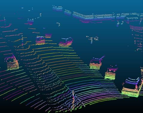
RangeRCNN
                      Range View
                                                                 Point View                 Bird’s Eye View       3D Proposal                  Box
                                                                                                                                            Refinement
      5×H×W
                        Encoder
                                                                                                                                            3D RoI
                                                                                                                                            Pooling
                        Decoder
      64×H×W
                                                                                                                  Classification            Confidence

                                                                                                                        Pointwise Feature

                 Range Image Backbone                                      RV-PV-BEV Module                               RPN                    RCNN

                                                             RangeDet

Fig. 2. Illustration of the framework of RangeRCNN. The input range image is visualized using the pseudocolor according to the range channel. After the
range image backbone, the high-level feature with 64 dimensions is extracted. We visualize it by t-SNE dimension reduction. The features extracted from
the range image are transferred to the point view and the bird’s eye view in turn. The region proposal network (RPN) is used to generate 3D proposals
from BEV. The 3D proposal and the pointwise feature are input into the 3D RoI pooling for proposal refinement. We name the one-stage network without
RCNN RangeDet, and name the whole two-stage framework RangeRCNN.

to easily overlap with each other. These two issues do not                         performance on the competitive KITTI 3D detection
exist in the 2D BEV space. Considering these properties, we                        benchmark and large-scale Waymo Open dataset.
propose a novel framework named RangeRCNN. First, we
extract features from the range image for its compact and                                          II. RELATED WORK
lossless representation. To better adapt the scale variation                  A. 3D Object Detection
of the range image, we utilize the dilated residual block                        3D Object Detection with Grid-based Methods. Most
which uses the dilated convolution [5] to achieve a more                      state-of-the-art methods in 3D object detection project the
flexible receptive field. Then, we propose the RV-PV-BEV                      point clouds to the regular grids. [6]–[9] directly projects
module to transfer the features extracted from the range view                 the original point clouds to the 2D bird’s eye view to
to the bird’s eye view. Because the high-level features are                   utilize the efficient 2D convolution for feature extraction.
effectively extracted, the influence of the quantization error                They also combine RGB images and other views for deep
caused by BEV is attenuated. The BEV mainly plays the                         feature fusion. [10] is a pioneering work in 3D voxel-based
role of anchor generation. Neither the range image nor the                    object detection. Based on [10], [1] increases the efficiency
bird’s eye image can explicitly supervise the height of the                   of the 3D convolution using sparse optimization. Several
3D bounding box. As a result, we propose to refine the 3D                     following methods [11]–[13] utilize the sparse operation [1],
bounding box using a two-stage RCNN. The point view in                        [2] to develop more accurate detectors. For the real-time
the RV-PV-BEV module does not only serve as the bridge                        3D object detector, [14] proposes the pillar-based voxel to
from RV to BEV, but also provides pointwise features for                      significantly improve the efficiency. However, the grid-based
RCNN refinement.                                                              methods suffer from information loss in the stage of initial
   In summary, the key contributions of this paper are as                     feature extraction. The sparsity issue of the point clouds
follows:                                                                      also limits the effective receptive field of 3D convolution.
  •   We propose the RangeRCNN framework which takes                          These problems will become more serious when processing
      the range image as the initial input to extract dense                   the large outdoor scene.
      and lossless features for fast and accurate 3D object                      3D Object Detection with Point-based Methods. Com-
      detection.                                                              pared to the grid-based methods, the point-based methods
  •   We design a 2D CNN utilizing dilated convolution to                     are limited by the high computation cost in early research
      better adapt the flexible receptive field of the range                  works. [15], [16] project 2D bounding boxes to the 3D space
      image.                                                                  to obtain 3D frustums and conduct the 3D object detection
  •   We propose the RV-PV-BEV module for transferring the                    in each frustum. [17], [18] directly process the whole point
      feature from the range view to the bird’s eye view for                  cloud using [19] and generate proposals in a bottom-up
      easier anchor generation.                                               manner. [20] introduces a vote-based 3D detector that is more
  •   We propose an end-to-end two-stage pipeline that uti-                   suitable to process indoor scenes. [21] uses a graph neural
      lizes a region convolutional neural network (RCNN) for                  network for point cloud detection. [22] proposes a fusion
      better height estimation. The whole network does not                    sampling strategy to speed up the point-based method.
      use 3D convolution or point-based convolution which                        3D Object Detection with Range Image. Compared to
      makes it simple and efficient.                                          the grid-based and point-based methods, fewer researchers
  •   Our proposed RangeRCNN achieves state-of-the-art                        utilize the range image in 3D object detection. [6] takes the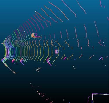
range image as one of its inputs. [3], [4] directly process the
range image for 3D object detection. However, the range
image based methods have not matched the performance                                                                    H×W×32

of the grid-based or point-based methods on the popular                                                                 H×W×64
KITTI dataset until now. [4] mentions that better results are                                                           H/2×W/2×128
achieved on the larger self-collected dataset. Recently, [23]                                                           H/4×W/4×128
has proposed the range conditioned dilated block for learning                                                           H/8×W/8×256
scale invariant features from the range image and achieves
                                                                                                                        H/16×W/16×256
the top performance on the large-scale Waymo Open dataset.
                                                                                                                        H/8×W/8×128
We think that the scale of the dataset is a secondary reason
for low accuracy. The main reason is that the range image                                                               H/4×W/4×128

is a good choice for extracting initial features, but not a                                                             H/2×W/2×64
good choice for generating anchors. In this paper, we design                                                            H×W×64
a better framework utilizing the range image representation
for 3D object detection.

B. Feature Learning on point clouds
                                                                  Fig. 3. Illustration of the backbone for the range image. The backbone is
   Recently, feature learning on point clouds has been studied    an encoder-decoder structure for extracting high-level features.
for different tasks, such as classification, detection and seg-
mentation. Among these tasks, the 3D semantic segmentation
task is chosen by many methods [2], [19], [24]–[26] as            easily obtain the BEV feature by projecting the 3D point to
the touchstone for evaluating the ability to extract features     the x-y plane. Since we have effectively extracted high-level
from point clouds. Early research was mainly focused on           features from the range image, BEV mainly plays the role
indoor scenes due to the lack of outdoor datasets. Se-            of proposal generation. This projection is therefore different
manticKITTI [27] is a recent semantic segmentation bench-         from projecting the 3D point to BEV at the beginning, which
mark for autonomous driving scenes. In the benchmark, [28]        is extremely dependent on the feature extraction from BEV.
proves the effectiveness of learning features from the range      We use a simple RPN to generate proposals from BEV
image for 3D semantic segmentation and simultaneously runs        and refine the proposals using the 3D RoI pooling module.
at a high speed. However, the value of the range image in the     We name the one-stage network without RCNN pooling
field of 3D object detection is far from being fully explored.    RangeDet, and name the two-stage framework RangeRCNN.
We believe that the range image can also provide rich and
useful information for the 3D object detection task.              B. Range Image Backbone
                                                                     Most existing datasets such as KITTI provide the point
             III. METHOD DESCRIPTION                              cloud as the LIDAR data format, so we need to convert the
   In section III-A, we present the network architecture of       points to the range image. As described in [28], the formula
our method. In section III-B, we introduce the backbone for       is as follows:
extracting features from the range image. In section III-C, we
introduce the RV-PV-BEV module for transferring features
                                                                          u
                                                                                            1
                                                                                                  − arctan(y, x)π −1 ] × w

                                                                                  =           2 [1                                      (1)
between different views. In section III-D, we utilize 3D RoI              v               [1 − (arcsin(z, r) + fdown )f −1 ] × h
pooling to refine the generated proposals. In section III-E,
we describe the loss function used in our network.                   where (x, y, z) represents the point coordinate in the 3D
                                                                  space.p(u, v) is the pixel coordinate in the range image.
A. Network Architecture                                           r = x2 + y 2 + z 2 is the range of each point. w and h
   Our proposed network is illustrated in Fig. 2. The 3D          are the predefined width and height of the range image. f =
point cloud is represented as the native range image, which is    fup +fdown is the vertical field-of-view of the LIDAR sensor.
fed into an encoder-decoder 2D backbone to extract features       For each pixel position, we encode its range, coordinate, and
efficiently and effectively. We upsample the deep feature         intensity as the input channel. As a result, the size of the
map to the original resolution of the range image using a         input range image is 5 × h × w. In [28], the categories of
decoder in order to retain more spatial information. We then      semantic segmentation are labeled for all points, so the range
transfer features from the range image to each point. We          image contains the 360-degree information. The LIDAR used
do not extract features based on the point view using the         by the KITTI dataset is the Velodyne 64E LIDAR with
point-based convolution [19], [24]. Actually, the point view      64 vertical channels. Each channel generates approximately
has two functions. First, it serves as the bridge from the        2000 points. In their task, therefore, h and w are respectively
range image to the bird’s eye image. Second, it provides          set as 64 and 2048. In the KITTI 3D detection task, the
the pointwise feature to the 3D RoI pooling module for            LIDAR and the camera are jointly calibrated. Only the
refining the proposals generated by the region proposal           objects in the front view of the camera are labeled; this view
network (RPN). After obtaining the pointwise feature, we can      represents approximately 90 degrees of the whole scene.
H×W×C
Conv 3×3
Dilate=1 Conv 3×3
H× W× 3C
Conv
H× W× C
Dilate=2 Output
Input 1×1
H×W×Cin H×W×C C +
Conv 3×3
Dilate=3
H×W×C
(a) Range Image (b) Bird’s Eye Image
(a) Dilated Residual Block
Fig. 5. Comparison of the range image (left) and the bird’s eye im-
Skip age (right). The bounding boxes in the range image differs notably in scale
Connection and easily overlap with each other. In contrast, the bounding boxes in the
H/2× W/2× Cin
bird’s eye image maintain similar size and do not have overlapping areas.
H\2× W\2× C
H× W× Cin
H× W× Cin
Conv Up
Dropout sample
DRB
DRB
1×1
C
Pooling
from the encoder. The concantenated feature is then input
to DRB. The size of the final output features (visualized in
(b) Dilated Downsample Block (c) Dilated Upsample Block
Fig. 3 by t-SNE) extracted from the range image is the same
Fig. 4. Illustration of the layer structure. (a) Dilated residual block (DRB).
size as the input with 64 dimensions.
(b) Dilated downsample block for the encoder. (c) Dilated upsample block C. RV-PV-BEV Module
for the decoder.
The range image representation is suitable for feature
extraction by utilizing the 2D convolution. However, it is
difficult to assign anchors in the range image plane due to
Additionally, some vertical channels are filtered by the FOV
the large scale variation. The severe occlusion also makes
of the camera. We thus set h = 48 and w = 512, which
it difficult to remove redundant bounding boxes in the Non-
is sufficient to contain the front view scene. The size of the
Maximum Suppression (NMS) module. Fig. 5 shows a typi-
range images used for the KITTI dataset is 5 × 48 × 512.
cal example. The size of the bounding boxes varies greatly in
The Waymo Open dataset provides range images with the
the range image. Some bounding boxes have a large overlap.
size of 64 × 2650 as the LIDAR data format. Therefore, we
In contrast, these bounding boxes have a similar shape in the
can directly use it without any extra conversion.
BEV plane because most cars are of similar size. It is also
The backbone for the range image is illustrated in Fig. 3. impossible for different cars to overlap with each other in
The 2D backbone for extracting features from the range the BEV place even though they are very close. We therefore
image is an encoder-decoder structure. The size of the feature think that it is more suitable to generate anchors in the BEV
map is given in the figure. The input is downsampled in plane. Thus, we transfer the feature extracted from the range
the encoder by six dilated downsample blocks (shown in image to the bird’s eye image.
Fig. 4(b)), then gradually upsampled in the decoder by four For each point, we record its corresponding pixel coor-
corresponding dilated upsample blocks (shown in Fig. 4(c)). dinates in the range image plane, so we can obtain the
The range image provides dense and compact representation pointwise feature by indexing the output feature of the range
for utilizing the 2D CNN but simultaneously presents the image backbone. Then, we project the pointwise feature to
scale variation issue. The scales of objects with different the BEV plane. For points corresponding with the same pixel
distances exhibit significant differences. To better adapt in the BEV image, we use the average pooling operation
different scales and obtain a more flexible receptive field, to generate the representative feature for the pixel. Here the
we design the dilated residual block (DRB), which inserts point view only serves as the bridge to transfer features from
the dilated convolution into the normal residual block. In the range image to the BEV image. We do not use the point-
this block (Fig. 4(a)), three 3 × 3 convolutions with different based convolution to extract features from points.
dilated rates {1, 2, 3} are applied to extract features with Discussion. Different from projecting point clouds to the
different receptive fields. The outputs of the three dilated BEV plane at the beginning of the network [6], [7], we
convolutions are concatenated followed by a 1 × 1 convo- perform the projection after extracting high-level features.
lution to fuse the features with different receptive fields. A If projecting at the beginning, the BEV serves as the main
residual connection is used to add the fused feature and the feature extractor. The information loss caused by the dis-
input feature. In the dilated downsample block (Fig. 4(b)), cretization leads to inaccurate features. In our framework,
we first use a 1 × 1 convolution to extract features across the BEV primarily plays the role of anchor generation. As
channels. Then the feature is input to DRB to extract features we have extracted features from the lossless range image, the
with a flexible receptive field. The dropout operation and the quantization error caused by the discretization has a minor
pooling operation are used for better generalization perfor- influence. Experiments show the superiority of our methods
mance and downsampling the feature map, respectively. In compared with those methods projecting at the beginning.
the first two blocks of the encoder, we do not use the pooling
operation. In the dilated upsample block (Fig. 4(c)), we first D. 3D RoI Pooling
use the bilinear interpolation to upsample the feature map. Based on the bird’s eye image, we generate 3D proposals
A skip connection is introduced to concatenate the feature using the region proposal network (RPN). However, neitherPointwise Feature IV. EXPERIMENTS
In this section, we evaluate our proposed RangeRCNN
Confidence
on the challenging KITTI dataset [33] and the large-scale
. Waymo Open dataset [34].
Flatten FC Dataset. The KITTI dataset [33] contains 7481 training
. samples and 7518 test samples. We follow the general split
. of 3712 training samples and 3769 validation samples. The
Box KITTI dataset provides a benchmark for 3D object detection.
Refinement We compare our proposed RangeRCNN with other state-of-
3D Proposal
the-art methods on this benchmark.
The Waymo Open dataset [34] provides 798 training
Fig. 6. Illustration of the 3D RoI pooling. The blue box is the 3D proposal. sequences and 202 validation sequences. Each sequence
It is divided into the regular grids along three aligned axes. Each grid obtains
the feature from the aforementioned point view. The max pooling operation contains 200 frames within 20 seconds. Specifically, this
is applied to pool multiple point features within a grid. All 3D grids are dataset provides the point clouds in the form of the range
flattened to a vectorized feature. Several fully connected layers are applied image, so we directly obtain the raw range image and do
to predict the refined boxes and the confidences.
not need to convert the point clouds to the range image.
A. Implementation Details
the range image nor the bird’s eye image explicitly learns Network Details. For the KITTI dataset, the size of the
features along the height direction of the 3D bounding box, input range image is 5 × 48 × 512 as mentioned above. For
which causes our predictions to be relatively accurate in the the Waymo Open dataset, the size of the range image is
BEV plane, but not in the 3D space. As a result, we want 6 × 64 × 2650, where 64 indicates 64 lasers and 2650 means
to explicitly utilize the 3D space information. We conduct that each laser has 2650 points. The LIDAR of the Waymo
a 3D RoI pooling based on the 3D proposals generated Open dataset has a 360 degree field of view instead of 90
by RPN. The proposal is divided into a fixed number of degrees as the KITTI dataset. The range image backbone for
grids. Different grids contain different parts of the object. the two datasets is described in Sec. III-B.
As these grids have a clear spatial relationship, the height For the KITTI dataset, the range of BEV is within
information is encoded among their relative positions. We [0, 69.12]m for the x-axis and [−39.68, 39.68]m for the y-
directly vectorize these grids from three dimensions to one axis. The resolution of BEV is 0.162 m2 , so the initial
dimension sorted by their 3D positions (illustrated in Fig. 6). spatial size of BEV is 496 × 432. We use three convolution
We apply several fully connected layers to the vectorized blocks to downsample the BEV to 248 × 216, 124 × 108
features and predict the refined bounding boxes and the and 62 × 54, and upsample the three sizes to 248 × 216.
corresponding confidences. The three features with the same size are then concatenated
along the channel axis. For the Waymo Open dataset, the
E. Loss Function range of BEV is within [−75.52, 75.52]m for the x-axis and
The whole network is trained in end-to-end fashion. The [−75.52, 75.52]m for the y-axis. The resolution of BEV is
loss contains two main parts: the region proposal network 0.322 m2 , so the initial spatial size of BEV is 472 × 472,
loss Lrpn and the region convolutional neural network loss which is slightly different from the size of 496 × 432 for the
Lrcnn , which is similar to [1], [11], [13]. The RPN loss KITTI dataset. The aforementioned concatenated features are
Lrpn includes the focal loss Lcls for anchor classification, the input to the RPN network for generating 3D proposals.
smooth-L1 loss Lreg for anchor regression and the direction In the two-stage RCNN, the 3D proposal generated by the
classification loss Ldir for orientation estimation [1]: RPN is divided into a fixed number of grids along with the
local coordinate system of the 3D proposal. The spatial shape
Lrpn = Lcls + αLreg + βLdir (2) is set as 12 × 12 × 12. We reshape the 12 × 12 × 12 grids
to a vectorized format with dimension of 123 × C, where C
where α is set to 2 and β is set to 0.2 empirically. We use
is the feature dimension of each grid. The feature of each
the default parameters for focal loss [29]. The smooth-L1
grid is obtained from the point features. C is equal to 64.
loss regresses the residual value relative to the anchor [1].
If multiple points fall within the same grid, the max pooling
The RCNN loss includes the confidence prediction loss is used. Three fully connected layers are then applied to the
Lscore guided by the IoU [11], the smooth-L1 loss Lreg for vectorized feature. Finally, the confidence branch and the
refining proposals and the corner loss Lcorner [15]: refinement branch are used to output the final result.
Lrcnn = Lscore + Lreg + Lcorner (3) Training and Inference Details. We implement the
proposed RangeRCNN with PyTorch1.3. The network can be
The total training loss is the sum of the above losses: trained in an end-to-end fashion with the ADAM optimizer.
For the KITTI dataset, we train the entire network with the
Ltotal = Lrpn + Lrcnn (4) batch size of 32 and learning rate of 0.01 for 80 epochs on 8
NVIDIA Tesla V100 GPUs, which takes approximately 1.5Fig. 7. Visualization of our predictions on the KITTI dataset.
TABLE I
P ERFORMANCE COMPARISON WITH PREVIOUS METHODS ON THE KITTI ONLINE TEST SERVER . T HE AP WITH 40 RECALL POSITIONS (R40) IS USED
TO EVALUATE THE 3D OBJECT DETECTION AND BEV OBJECT DETECTION .
3D BEV
Method Reference Modality
Easy Moderate Hard Easy Moderate Hard
Multi-Modality:
MV3D [6] CVPR 2017 RGB+LIDAR 74.97 63.63 54.00 86.62 78.93 69.80
ContFuse [9] ECCV 2018 RGB+LIDAR 83.68 68.78 61.67 94.07 85.35 75.88
AVOD-FPN [7] IROS 2017 RGB+LIDAR 83.07 71.76 65.73 90.99 84.82 79.62
F-PointNet [15] CVPR 2018 RGB+LIDAR 82.19 69.79 60.59 91.17 84.67 74.77
UberATG-MMF [8] CVPR 2019 RGB+LIDAR 88.40 77.43 70.22 93.67 88.21 81.99
EPNet [30] ECCV 2020 RGB+LIDAR 89.91 79.28 74.59 94.22 88.47 83.69
LIDAR-only:
PointRCNN [17] CVPR 2019 Point 86.96 75.64 70.70 92.13 87.39 82.72
Point-GNN [21] CVPR 2020 Point 88.33 79.47 72.29 93.11 89.17 83.90
3D-SSD [22] CVPR 2020 Point 88.36 79.57 74.55 92.66 89.02 85.86
SECOND [1] Sensors 2018 Voxel 83.34 72.55 65.82 89.39 83.77 78.59
PointPillars [14] CVPR 2019 Voxel 82.58 74.31 68.99 90.07 86.56 82.81
3D IoU Loss [31] 3DV 2019 Voxel 86.16 76.50 71.39 91.36 86.22 81.20
Part-A2 [11] TPAMI 2020 Voxel 87.81 78.49 73.51 91.70 87.79 84.61
Fast Point R-CNN [32] ICCV 2019 Voxel+Point 85.29 77.40 70.24 90.87 87.84 80.52
STD [18] ICCV 2019 Voxel+Point 87.95 79.71 75.09 94.74 89.19 86.42
SA-SSD [12] CVPR 2020 Voxel+Point 88.75 79.79 74.16 95.03 91.03 85.96
PV-RCNN [13] CVPR 2020 Voxel+Point 90.25 81.43 76.82 94.98 90.65 86.14
LaserNet [4] CVPR 2019 Range - - - 79.19 74.52 68.45
RangeRCNN (ours) - Range 88.47 81.33 77.09 92.15 88.40 85.74
TABLE II
0.01 for 30 epochs on 8 NVIDIA Tesla V100 GPUs, which
RUNTIME ANALYSIS OF STATE - OF - THE - ART TWO - STAGE DETECTORS .
takes approximately 70 hours. We adopt the cosine annealing
learning rate strategy for the learning rate decay.
PointRCNN PartA2 PV-RCNN RangeRCNN
FPS (Hz) 12 13 10 22 For the KITTI dataset, we use the data augmentation
strategy similar to [1], [11], including random flipping along
the x-axis, random global scaling with a scaling factor
sampled from [0.95, 1.05], random global rotation around
hours. For the large-scale Waymo Open dataset, we train the the vertical axis with a sampled angle from [− π4 , π4 ], and
entire network with the batch size of 32 and learning rate of ground-truth sampling augmentation to randomly ”paste”TABLE III
P ERFORMANCE COMPARISON WITH PREVIOUS METHODS ON THE LEVEL 1 VEHICLE OF THE WAYMO VALIDATION SET.
3D mAP 3D mAPH
All 0-30m 30-50m 50-75m All 0-30m 30-50m 50-75m
LaserNet [4] 52.11 70.94 52.91 29.62 50.05 68.73 51.37 28.55
PointPillars [14] 56.62 81.01 51.75 27.94 - - - -
RCD [23] 68.95 87.22 66.53 44.53 68.52 86.82 66.07 43.97
PV-RCNN [13] 70.30 91.92 69.21 42.17 69.69 91.32 68.53 41.31
RangeRCNN (ours) 75.43 92.01 74.27 54.23 74.97 91.52 73.77 53.54
some new ground-truth objects to current training scenes. For C. 3D Detection on the Waymo Open Dataset
the Waymo Open dataset, we discuss the data augmentation Metrics. The mean average precision (mAP) and the
strategy in Sec. IV-D. mean average precision weighted by heading (mAPH) are
For RCNN, we choose 128 proposals with a 1:1 ratio adopted as the metrics of this dataset. The IoU threshold
for positive and negative samples during training. During for vehicles is set as 0.7. The detection performances with
inference, we retain the top 100 proposals according to the different object distances are reported. The dataset divides
confidence with the NMS threshold 0.7. We apply the 3D the objects into two difficulty levels based on the number
NMS to the refined bounding boxes with a threshold of 0.1 of points within the 3D boxes. Level 1 includes at least
to generate the final result. five points with the 3D box and Level 2 includes at least
one point. As few previous methods report their Level 2
B. 3D Detection on the KITTI Dataset performance, we compare RangeRCNN with state-of-the-art
Metrics. The detection result is evaluated using the mean methods with respect to Level 1.
average precision (mAP) with the IoU threshold 0.7. For the Performance. Table III shows that RangeRCNN out-
official test benchmark, the mAP with 40 recall positions is performs previous methods by a large margin. The Waymo
used. We report the performance of 3D detection and BEV dataset directly provides the range image without the require-
detection in Table I. ment of additional conversion, so the quality of the range
Performance. We submit our results to the online bench- image is better than that of the KITTI dataset. RangeR-
mark for comparison with other state-of-the-art methods. For CNN has the ability to extract rich information for distant
evaluating the test set, we use all provided labeled samples objects. For objects within [0, 30]m, the performance of
to train our model. Table I reports the results evaluated on RangeRCNN is similar to that of PV-RCNN. For objects
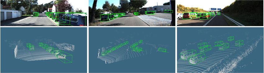
the KITTI online test server. Fig. 7 shows the qualitative within [30, 50]m and [50, 75]m, RangeRCNN performs much
results. Our RangeRCNN outperforms almost all previous better than PV-RCNN. The farther away the object is, the
approaches except PV-RCNN [13] on the commonly used greater the advantage of our method over other methods.
moderate level for 3D car detection. We surprisingly observe RangeRCNN outperforms RCD which also utilizes the range
that our method achieves the highest accuracy for the hard image representation. RCD only operates on the range image
level. We think that the performance is beneficial to two which does not utilize the ability of BEV to generate anchors.
aspects. First, some hard examples are very sparse in the The performance of RangeRCNN on this large-scale dataset
3D space, but they have more obvious features in the range shows the large potential of the range image based method.
image thanks to the compact representation. These objects
can thus be detected using the range image representation. D. Discussion on Data Augmentation of Range Image.
Second, RCNN further refines the 3D position of the bound- For the KITTI dataset, it does not directly provide the
ing box, which boosts the 3D performance. The ablation range image, so we need to convert the points to the range
study also proves the value of RCNN. image. In this dataset, we first perform data augmentation on
Runtime Analysis. To provide a fair runtime compari- the points similar with [1], [11]. Then we convert the aug-
son, we run several representative two-stage methods with mented points to the range image. Although the augmented
the same device (NVIDIA V100 GPU). The comparison range image no longer strictly adheres to the scanning char-
is shown in Table. II. The proposed RangeRCNN runs at acteristic of the rotating LIDAR, the augmentation strategy
22 fps, which is much faster than the point-based PointR- brings an improvement in accuracy.
CNN and the voxel-based PartA2 and PV-RCNN. The high For the Waymo Open dataset, the data augmentation
computation performance is beneficial from the compact pipeline is a little bit different from that of the KITTI
representation of the range image and the efficiency of 2D dataset. Since the Waymo dataset provides the range image
convolution. Research on the range image can promote real- representation, we directly flip and rotate the range image,
time 3D object detection. and scale the point coordinates stored in the channel of(a) Range image before cut-and-paste
(b) Objects before cut-and-paste
(c) Range image after cut-and-paste
(d) Objects after cut-and-paste
Fig. 8. Illustration of the cut-and-paste strategy for the Waymo Open dataset. Vehicles, Pedestrians and Cyclists are marked blue, green and red, respectively.
TABLE IV TABLE V
C OMPARISON OF THE ONE - STAGE MODEL R ANGE D ET AND THE C OMPARISON OF DIFFERENT POOLING SIZES IN {6, 8, 10, 12, 14}. T HE
TWO - STAGE MODEL R ANGE RCNN. T HE AP WITH 40 RECALL AP WITH 40 RECALL POSITIONS (R40) IS USED .
POSITIONS (R40) IS USED .
3D BEV
Method
3D BEV Easy Moderate Hard Easy Moderate Hard
Method
Easy Moderate Hard Easy Moderate Hard RangeRCNN-6 89.55 82.33 80.01 92.56 88.47 87.78
RangeRCNN-8 89.23 82.35 79.96 92.44 88.49 88.00
RangeDet 89.87 80.72 77.37 92.07 88.37 87.03
RangeRCNN-10 89.48 82.62 80.36 92.76 88.60 88.11
RangeRCNN 91.41 82.77 80.39 92.84 88.69 88.20
RangeRCNN-12 91.41 82.77 80.39 92.84 88.69 88.20
RangeRCNN-14 91.54 82.61 80.29 92.67 88.49 88.16
E. Ablation Study
In this section, we conduct the ablation study on the
the range image. One interesting operation is to apply the validation set of the KITTI dataset.
cut-and-paste strategy on the range image (illustrated in Effects of 3D RoI Pooling. As the entire framework is
Fig. 8). We first traverse the training data and read all two-stage, we compare the results of the one-stage model
annotated objects. For each point in the object, we store RangeDet and the two-stage model RangeRCNN to analyze
its 3D coordinate, intensity, elongation and corresponding the value of RCNN. From Table IV, we can find that
pixel coordinate on the range image plane. When training the RangeDet and RangeRCNN exhibit similar performances for
model, we randomly paste the object according to the pixel BEV detection. For 3D detection, RangeRCNN outperforms
coordinates to augment the original range image. In addition RangeDet by a large margin. The better 3D performance
to augment the range image, we also need to simultaneously comes from the 3D information encoded by 3D RoI pooling.
consider the corresponding changes and transformation for Effects of Grid Size in 3D RoI Pooling. We further
the 3D point coordinates. The improvement brought by the evaluate the influence of the grid size in 3D RoI pooling. We
cut-and-paste strategy depends on several factors. If we use compare a set of grid sizes in {6, 8, 10, 12, 14}. Table V
a small part of the whole Waymo Open dataset for training, shows the results. It can be found that the grid size exerts
the improvement will be more obvious, which means that no great influence on the metric. We choose 12 as the grid
this strategy is very effective with limited training data. size, which is a relatively better size.
For the category with much fewer labels such as cyclists,
the improvement will be much greater, which means that V. CONCLUSIONS
this strategy is helpful for some scarce categories. As the In this paper, we explore the potential of the range
Waymo Open dataset is large, if training with all data, this image representation and present a novel framework called
strategy hardly improves the accuracy of vehicles with large RangeRCNN for fast and accurate 3D object detection. By
amount of annotations. We believe that the augmentation combining the advantages of extracting lossless features on
strategy is very useful for future reserach based on range the range image and generating high-quality anchors on
image. Through the range image based data augmentation, the bird’s eye image, our method achieves state-of-the-art
the preprocessing pipeline of the range image based method performance on the KITTI dataset and the Waymo Open
is almost equivalent to the voxel based method and the point dataset while maintaining high efficiency. The compact rep-
based method. Detailed experiments and analysis will be resentation of the range image provides more possibilities
provided in the future version. for real-time 3D object detection in large outdoor scenes.R EFERENCES [21] W. Shi and R. Rajkumar, “Point-gnn: Graph neural network for 3d
object detection in a point cloud,” in Proceedings of the IEEE/CVF
[1] Y. Yan, Y. Mao, and B. Li, “Second: Sparsely embedded convolutional Conference on Computer Vision and Pattern Recognition, 2020, pp.
detection,” Sensors, vol. 18, no. 10, p. 3337, 2018. 1711–1719.
[2] B. Graham, M. Engelcke, and L. van der Maaten, “3d semantic [22] Z. Yang, Y. Sun, S. Liu, and J. Jia, “3dssd: Point-based 3d single
segmentation with submanifold sparse convolutional networks,” in stage object detector,” in Proceedings of the IEEE/CVF Conference on
Proceedings of the IEEE Conference on Computer Vision and Pattern Computer Vision and Pattern Recognition, 2020, pp. 11 040–11 048.
Recognition, 2018, pp. 9224–9232. [23] A. Bewley, P. Sun, T. Mensink, D. Anguelov, and C. Sminchisescu,
[3] B. Li, T. Zhang, and T. Xia, “Vehicle detection from 3d lidar using “Range conditioned dilated convolutions for scale invariant 3d object
fully convolutional network,” in Proceedings of Robotics: Science and detection,” arXiv preprint arXiv:2005.09927, 2020.
Systems (RSS), 2016. [24] C. R. Qi, H. Su, K. Mo, and L. J. Guibas, “Pointnet: Deep learning
[4] G. P. Meyer, A. Laddha, E. Kee, C. Vallespi-Gonzalez, and C. K. on point sets for 3d classification and segmentation,” in Proceedings
Wellington, “Lasernet: An efficient probabilistic 3d object detector of the IEEE conference on computer vision and pattern recognition,
for autonomous driving,” in Proceedings of the IEEE/CVF Conference 2017, pp. 652–660.
on Computer Vision and Pattern Recognition (CVPR), June 2019, pp. [25] Y. Li, R. Bu, M. Sun, W. Wu, X. Di, and B. Chen, “Pointcnn: Con-
12 677–12 686. volution on x-transformed points,” in Advances in neural information
[5] L.-C. Chen, G. Papandreou, I. Kokkinos, K. Murphy, and A. L. Yuille, processing systems, 2018, pp. 820–830.
“Deeplab: Semantic image segmentation with deep convolutional nets, [26] B. Wu, A. Wan, X. Yue, and K. Keutzer, “Squeezeseg: Convolutional
atrous convolution, and fully connected crfs,” IEEE transactions on neural nets with recurrent crf for real-time road-object segmentation
pattern analysis and machine intelligence, vol. 40, no. 4, pp. 834– from 3d lidar point cloud,” in 2018 IEEE International Conference on
848, 2017. Robotics and Automation (ICRA). IEEE, 2018, pp. 1887–1893.
[6] X. Chen, H. Ma, J. Wan, B. Li, and T. Xia, “Multi-view 3d object [27] J. Behley, M. Garbade, A. Milioto, J. Quenzel, S. Behnke, C. Stach-
detection network for autonomous driving,” in 2017 IEEE Conference niss, and J. Gall, “Semantickitti: A dataset for semantic scene under-
on Computer Vision and Pattern Recognition (CVPR), 2017, pp. 6526– standing of lidar sequences,” in Proceedings of the IEEE International
6534. Conference on Computer Vision, 2019, pp. 9297–9307.
[7] J. Ku, M. Mozifian, J. Lee, A. Harakeh, and S. L. Waslander, “Joint [28] A. Milioto, I. Vizzo, J. Behley, and C. Stachniss, “Rangenet++:
3d proposal generation and object detection from view aggregation,” Fast and accurate lidar semantic segmentation,” in 2019 IEEE/RSJ
in 2018 IEEE/RSJ International Conference on Intelligent Robots and International Conference on Intelligent Robots and Systems (IROS).
Systems (IROS), 2018, pp. 1–8. IEEE, 2019, pp. 4213–4220.
[8] M. Liang, B. Yang, Y. Chen, R. Hu, and R. Urtasun, “Multi-task [29] T.-Y. Lin, P. Goyal, R. Girshick, K. He, and P. Dollár, “Focal loss
multi-sensor fusion for 3d object detection,” in Proceedings of the for dense object detection,” in Proceedings of the IEEE international
IEEE/CVF Conference on Computer Vision and Pattern Recognition conference on computer vision, 2017, pp. 2980–2988.
(CVPR), June 2019, pp. 7345–7353. [30] T. Huang, Z. Liu, X. Chen, and X. Bai, “Epnet: Enhancing point
[9] M. Liang, B. Yang, S. Wang, and R. Urtasun, “Deep continuous fusion features with image semantics for 3d object detection,” Proceedings
for multi-sensor 3d object detection,” in Proceedings of the European of the European Conference on Computer Vision (ECCV), 2020.
Conference on Computer Vision (ECCV), 2018, pp. 641–656. [31] D. Zhou, J. Fang, X. Song, C. Guan, J. Yin, Y. Dai, and R. Yang, “Iou
[10] Y. Zhou and O. Tuzel, “Voxelnet: End-to-end learning for point loss for 2d/3d object detection,” in 2019 International Conference on
cloud based 3d object detection,” in 2018 IEEE/CVF Conference on 3D Vision (3DV), 2019, pp. 85–94.
Computer Vision and Pattern Recognition, 2018, pp. 4490–4499. [32] Y. Chen, S. Liu, X. Shen, and J. Jia, “Fast point r-cnn,” in Proceed-
[11] S. Shi, Z. Wang, J. Shi, X. Wang, and H. Li, “From points to ings of the IEEE/CVF International Conference on Computer Vision
parts: 3d object detection from point cloud with part-aware and part- (ICCV), October 2019.
aggregation network,” IEEE Transactions on Pattern Analysis and [33] A. Geiger, P. Lenz, and R. Urtasun, “Are we ready for autonomous
Machine Intelligence, 2020. driving? the kitti vision benchmark suite,” in 2012 IEEE Conference
[12] C. He, H. Zeng, J. Huang, X.-S. Hua, and L. Zhang, “Structure aware on Computer Vision and Pattern Recognition. IEEE, 2012, pp. 3354–
single-stage 3d object detection from point cloud,” in Proceedings of 3361.
the IEEE/CVF Conference on Computer Vision and Pattern Recogni- [34] P. Sun, H. Kretzschmar, X. Dotiwalla, A. Chouard, V. Patnaik, P. Tsui,
tion, 2020, pp. 11 873–11 882. J. Guo, Y. Zhou, Y. Chai, B. Caine et al., “Scalability in perception
[13] S. Shi, C. Guo, L. Jiang, Z. Wang, J. Shi, X. Wang, and H. Li, “Pv- for autonomous driving: Waymo open dataset,” in Proceedings of the
rcnn: Point-voxel feature set abstraction for 3d object detection,” in IEEE/CVF Conference on Computer Vision and Pattern Recognition,
Proceedings of the IEEE/CVF Conference on Computer Vision and 2020, pp. 2446–2454.
Pattern Recognition, 2020, pp. 10 529–10 538.
[14] A. H. Lang, S. Vora, H. Caesar, L. Zhou, J. Yang, and O. Beijbom,
“Pointpillars: Fast encoders for object detection from point clouds,”
in Proceedings of the IEEE/CVF Conference on Computer Vision and
Pattern Recognition (CVPR), June 2019, pp. 12 697–12 705.
[15] C. R. Qi, W. Liu, C. Wu, H. Su, and L. J. Guibas, “Frustum
pointnets for 3d object detection from rgb-d data,” in 2018 IEEE/CVF
Conference on Computer Vision and Pattern Recognition, 2018, pp.
918–927.
[16] Z. Wang and K. Jia, “Frustum convnet: Sliding frustums to aggregate
local point-wise features for amodal 3d object detection,” in 2019
IEEE/RSJ International Conference on Intelligent Robots and Systems
(IROS), 2019, pp. 1742–1749.
[17] S. Shi, X. Wang, and H. Li, “Pointrcnn: 3d object progposal gener-
ation and detection from point cloud,” in Proceedings of the IEEE
Conference on Computer Vision and Pattern Recognition, 2019, pp.
770–779.
[18] Z. Yang, Y. Sun, S. Liu, X. Shen, and J. Jia, “Std: Sparse-to-dense
3d object detector for point cloud,” in Proceedings of the IEEE
International Conference on Computer Vision, 2019, pp. 1951–1960.
[19] C. R. Qi, L. Yi, H. Su, and L. J. Guibas, “Pointnet++: Deep hierar-
chical feature learning on point sets in a metric space,” in Advances
in Neural Information Processing Systems, 2017, pp. 5099–5108.
[20] C. R. Qi, O. Litany, K. He, and L. Guibas, “Deep hough voting for
3d object detection in point clouds,” in 2019 IEEE/CVF International
Conference on Computer Vision (ICCV), 2019, pp. 9276–9285.You can also read