Decentralized Localization in Homogeneous Swarms Considering Real-World Non-Idealities
←
→
Page content transcription
If your browser does not render page correctly, please read the page content below
IEEE ROBOTICS AND AUTOMATION LETTERS, VOL. 6, NO. 4, OCTOBER 2021                                                                                          6765

Decentralized Localization in Homogeneous Swarms
      Considering Real-World Non-Idealities
                                                   Hanlin Wang            and Michael Rubenstein

   Abstract—This letter presents a decentralized algorithm that
allows a swarm of identically programmed agents to cooperatively
estimate their global poses using local range and bearing measure-
ments. The design of our algorithm explicitly considers the phase
asynchrony of each agent’s local clock, moreover, the execution of
our algorithm does not require each agent to actively keep the same
neighbors over time. A theoretical analysis about the effect of each
agent’s sensing noise and communication loss is given, in addition,
we validate the presented algorithm via experiments running on a
swarm of up to 256 simulated robots and a swarm of 100 physical
robots. The results from the experiments show that the presented
algorithm allows each agent to estimate its global pose quickly and
reliably. Video of 100 robots executing the presented algorithm as
well as supplementary material can be found in [1] and [2].
  Index Terms—Swarms, distributed robot systems, sensor                            Fig. 1. (Top) 100 Coachbot V2.0 robots are placed in three patterns; (Bottom)
networks.                                                                          The robots’ position estimates obtained via the proposed algorithm.

                            I. INTRODUCTION                                        and relative measurements. Decentralized methods can be cat-
                                                                                   egorized into two types: progressive methods [12]–[14], [18],
      OCALIZATION plays an important role in swarm systems.
L     In many collective tasks, such as shape formation [3]–[5],
shepherding [6], and more [7], it is valuable to have each agent
                                                                                   [23] and concurrent methods [16]. In progressive methods, each
                                                                                   agent has two possible states: localized and unlocalized. The
                                                                                   unlocalized agents will localize themselves using the inter-agent
know its pose in a global coordinate system.
                                                                                   measurements and the pose estimates from their already lo-
  Previous methods can be categorized into centralized meth-
                                                                                   calized neighbors, then, these unlocalized agents will become
ods [3], [8]–[10], and decentralized methods [11]–[21]. In
                                                                                   localized agents and their pose estimates will later be used by
centralized methods, agents obtain their poses from a central
                                                                                   their unlocalized neighbors. It was shown in [12], [13], [23]
controller [8], [9], or a pre-setup external infrastructure [3], [10].
                                                                                   that with certain amount of pre-localized anchoring agents, it
This type of method can work well in well-controlled environ-
                                                                                   is possible to accurately localize a densely placed swarm using
ments, but cannot easily be deployed in unknown environments,
                                                                                   the local information only. However, each agent’s position error
and suffer from the single point of failure problem [22].
                                                                                   will accumulate over its communication hops away from the
  Decentralized methods, in contrast, are inherently more scal-
                                                                                   anchoring agents. In addition, this type of method requires an
able and more robust to failures. Here, it is assumed that each
                                                                                   additional phase to set certain agents as anchoring agents. The
agent is able to communicate with nearby agents. In addition,
                                                                                   beacon-free solutions are proposed in [14], [18]. In [14], agents
each agent can measure its distance [11]–[16], bearing [17],
                                                                                   use inter-agent distance information to organize robust quads
[18], or both [19]–[21] relative to its neighbors. The agents
                                                                                   with their nearby agents. The adjacent robust quads can recover
will estimate their global poses using the local communication
                                                                                   their relative positions using the information from the set of
                                                                                   agents in common between two quads. However, it has not been
   Manuscript received February 24, 2021; accepted June 23, 2021. Date of          shown that this method can estimate agent’s orientation. The
publication July 7, 2021; date of current version July 22, 2021. This letter       work presented in [18] allows agents to estimate their orienta-
was recommended for publication by Associate Editor M. Ani Hsieh and               tion using the inter-agent bearing information, in addition, this
Editor A. Prorok upon evaluation of the Reviewers’ comments. This work was         methods is also able to localize only a subset of the agents in
supported by the National Science Foundation under Grant CMMI-2024774.
(Corresponding author: Hanlin Wang.)                                               the swarm. However, the coordinate system established by this
   Hanlin Wang is with the Department of Computer Science, North-                  method is scale-free, requiring an additional step to recover the
western University, Evanston, IL 60601 USA (e-mail: hanlinwang2015@                coordinate system’s scale [24].
u.northwestern.edu).                                                                  Different from the progressive methods, in concurrent meth-
   Michael Rubenstein is with the Department of Computer Science and the
Department of Mechanical Engineering, Northwestern University, Evanston, IL
                                                                                   ods [16], [25], [26], agents do not explicitly hold a Boolean state
60208 USA (e-mail: rubenstein@northwestern.edu).                                   of being localized or unlocalized. Instead, all the agents will
   This letter has supplementary downloadable material available at https://doi.   constantly and cooperatively refine their pose estimates using
org/10.1109/LRA.2021.3095032, provided by the authors.                             their local measurements. The concurrent methods are generally
   Digital Object Identifier 10.1109/LRA.2021.3095032                              more robust to sensing noise, in addition, these types of methods

                         2377-3766 © 2021 IEEE. Personal use is permitted, but republication/redistribution requires IEEE permission.
                                       See https://www.ieee.org/publications/rights/index.html for more information.

           Authorized licensed use limited to: Northwestern University. Downloaded on July 28,2021 at 21:03:10 UTC from IEEE Xplore. Restrictions apply.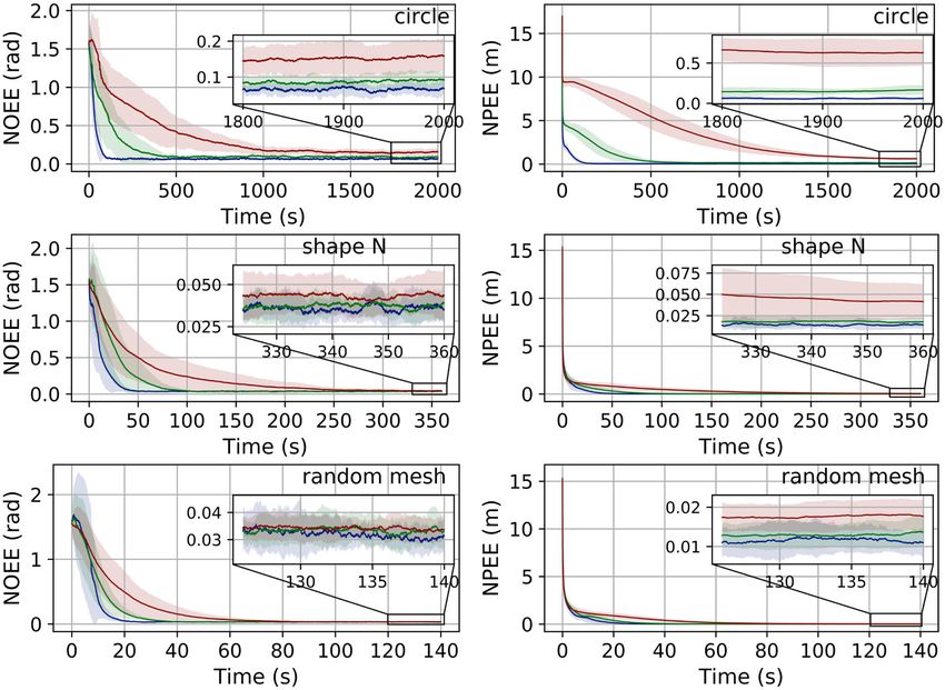
6766                                                                                IEEE ROBOTICS AND AUTOMATION LETTERS, VOL. 6, NO. 4, OCTOBER 2021

                                                                                  0 < λ < 1. In addition, we assume the agent’s bearing and range
                                                                                  sensor is noisy, that is: let Bij and dij be agent aj ’s actual
                                                                                  bearing angle and distance measured by agent ai , respectively.
                                                                                  When agent ai attempts to measure those two quantities, the
                                                                                  actual measurements returned from the sensor will be two ran-
                                                                                  dom variables Bˆij = Bij + B 2π and dˆij = dij + d , where
                                                                                  ·2π := · + 2π π−·
                                                                                                    2π  denotes the 2π modulus operator [27],
Fig. 2. Graphical illustration of the agent’s sensing capability. The red and     which is an operator that wraps an angle from the real space
green arrow lines are each agent’ local coordinate frame, where red arrow line
is the x-axis.
                                                                                  to the interval (−π, π], and B ∼ N (0, σB2 ), d ∼ N (0, σd2 ) are
                                                                                  two independent zero-mean Gaussian random variables.

are more robust to the unexpected external disturbances such as                   B. Problem Statement
the removal or the addition of the agents. One drawback for this
type of method is that, compared to the progressive methods, the                     Our task is to design an algorithm that estimates each agent’s
concurrent methods’ commutation cost is often more expensive,                     pose in a global frame using local information only. In our
as each agent needs to frequently exchange its pose estimates                     algorithm, this task is achieved by forcing agents to constantly
with its neighbors.                                                               and cooperatively refine their pose estimates to reduce the in-
   In this letter, we present a fully decentralized concurrent                    consistency between their pose estimates and the local mea-
localization algorithm for localizing a swarm of identically pro-                 surements. The global pose estimation will occur when each
grammed agents. We assume that each agent can talk to nearby                      agent’s pose estimate becomes consistent with its local mea-
agents, and that when an agent receives a message, it can measure                 surements and its neighbors’ pose estimates. More formally, let
the transmitter’s bearing and distance. The agents will estimate                  A = [a1 , a2 , . . ., an ] be a set of n agents, we use the undirected
their global poses by cooperatively minimizing the disagree-                      graph G = {A, E} to describe the network’s communication
ment between local measurements and their pose estimates. The                     topology. For a pair of agents ai and aj , (i, j) ∈ E iff they are
novelty of our algorithm is that: The design of our algorithm                     located in each other’s communication/sensing range R, and
explicitly considers the phase asynchrony of each agent’s local                   for each agent ai , the set of all the agents located in its com-
clock, moreover, the execution of our algorithm does not require                  munication range is denoted as Ni = {aj |aj ∈ A, (i, j) ∈ E}.
each agent to actively keep the same neighbors over time, which                   To simplify the description and analysis of the algorithm, it is
helps to avoid unnecessary communication overhead and makes                       assumed that G is always connected. In addition, we assume
our algorithm more flexible. A theoretical analysis about the                     that each agent is stationary. Note that the assumption of each
effect of each agent’s sensing noise and communication loss is                    agent being stationary is only for the sake of analysis, the actual
given, in addition, the algorithm’s performance is thoroughly                     execution of our algorithm does not require this assumption. An
investigated via experiments running on a swarm of up to 256                      example of the algorithm working in the situation where the
simulated agents as well as a swarm of 100 physical robots.                       swarm’s communication topology is dynamically changing is
The results from those experiments show that our algorithm                        shown in Section V-C. Each agent ai uses the vector [θix , θiy ] and
is able to reliably localize the swarms with different sizes and                  vector [xi , yi ] to describe its orientation estimate and position es-
configurations.                                                                   timate, respectively, where θi = arctan 2(θiy , θix ) is the agent’s
                                                                                  orientation estimate, and [xi , yi ] is the agent’s estimate of its xy
                           II. PRELIMINARIES                                      position. The agents will estimate their pose by cooperatively
                                                                                  solving the following two problems:
   In this section, we introduce the agent model used in the design                  Problem 1: (Orientation Estimation): Let Wij be the true
as well as the analysis of the algorithm, and formally state the                  orientation difference between two agent ai and aj , we define
decentralized localization problem.                                               the swarm’s orientation estimate error fo as:
                                                                                                                                      2
                                                                                  1   1            1        cos(W ), − sin(W ) θ          θjx
A. Agent Model                                                                                                     ij          ij      ix
                                                                                                                                          −
                                                                                  4 a ∈A a ∈N |Ni | |Nj |     sin(Wij ), cos(Wij )    θiy   θjy
   We assume that the agents are placed on a 2D plane. Each                          i     j   i                                                                  2

agent holds a local coordinate frame where the local coordinate                   The task is to find each agent ai ’s orientation estimate          [θix∗ , θiy∗ ]
frame’s origin is fixed on the center of the agent and the x-axis’                that minimizes the objective fo above.
direction is aligned with the agent’s heading. We assume each                         Problem 2: (Position Estimation): For each agent ai , given
agent’s clock has the same frequency but can be asynchronous                      ai ’s orientation estimate θi = arctan 2(θiy , θix ), we define the
in phase. In addition, it is assumed that each agent has a locally                swarm’s position estimate error fp as:
unique ID. We assume each agent is able to broadcast messages                                                                           2
to all agents within its communication range R. Moreover, when                     1   1 1                 xi +dij cos(Bij +θi ) − xj

an agent ai receives a message from a neighbor aj , the agent ai                   4
                                                                                                  |Ni | |Nj | yi            sin(Bij +θi )     yj 2
                                                                                      ai ∈A aj ∈Ni
is able to sense the transmitter aj ’s relative bearing angle Bij and
the distance dij . See Fig. 2 for a graphical illustration of agent’s             The task is: given each agent’s orientation estimate obtained
sensing capabilities. One real-world example that fits our agent                  from problem 1, find each agent ai ’s position estimate [x∗i , yi∗ ]
model is the Bluetooth 5.1 AOA device [20].                                       that minimizes the objective fp above.
   In order to make our agent model more realistic, we assume                        The objective fo and fp can be intuitively interpreted as
the inter-agent communication channel is lossy, that is: for                      the normalized sum of the inconsistency between each pair of
an agent ai , when a nearby neighbor aj transmits a message,                      agents’ pose estimates and their distance, orientation difference,
ai will receive this message with a probability of λ, where                       as well as bearings relative to each other.

         Authorized licensed use limited to: Northwestern University. Downloaded on July 28,2021 at 21:03:10 UTC from IEEE Xplore. Restrictions apply.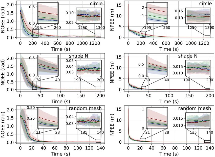
WANG AND RUBENSTEIN: DECENTRALIZED LOCALIZATION IN HOMOGENEOUS SWARMS CONSIDERING REAL-WORLD NON-IDEALITIES                                              6767

C. From Bearing Angle to Orientation Difference
   One can see that in order to solve problem 1, each agent
ai needs to be able to measure nearby agent aj ’s orientation
difference Wij . On the other hand, as stated in Section II-A,
agent ai is not able to measure the neighbor aj ’s orientation
difference directly. It was shown in [18] that, for two agents
ai and aj , given their bearing angles in the other’s local frame
Bji and Bij , their orientation difference Wij can be explicitly
written as: Wij = Bij − Bji + π2π .

                           III. APPROACH
   As we briefly discussed in Section II-B, in our algorithm,
the agents will actively refine their pose estimates to minimize
the objective fo and fp . When doing so, each agent will treat
the objective fo and the objective fp separately: each agent
ai updates its orientation estimate [θix , θiy ] only according
to objective fo (Algorithm 1, Line 20-21), and then uses the
obtained orientation estimate [θix , θiy ] to calculate objective fp
so as to update its position estimate [xi , yi ] (Algorithm 1, Line
22-24).
   In the algorithm, each agent will consistently broadcast its
current pose estimate to the neighbors at a fixed frequency of
f (Algorithm 1, Line 28), meanwhile, at the same frequency,
it will periodically update its pose estimate using the messages
received (Algorithm 1, Line 10-26). For each agent, the message
received from another agent can be characterised by a 3-tuple
msg = (data, B̂, d),   ˆ where data is the payload of the message,
B̂ is the measurement of transmitter’s bearing angle, and dˆ is the
measurement of transmitter’s distance. See Algorithm 1 for the
detailed pseudo code of the proposed algorithm, and below is a
detailed description of the main variables used in the algorithm:
   • id: the agent’s id, which is locally unique;
   • α, β: the variables to control the step size of the update of              by aj . On the other hand, the second measurement B̂ji cannot be
the agent’s pose estimate;                                                      obtained by ai via local sensing directly. In order to allow each
   • msg_buff: the buffer to store the messages received in the                 agent to obtain its own bearing angle measured by its neighbors,
latest f1 amount of time;                                                       the agents will cooperatively execute a “random echo” protocol:
                                                                                for each agent in the swarm, every time when forging msg_out,
   • last_check: the variable to record when was the last time                  it will first uniformly and randomly select a message echo_msg
the agent transmitted a message;                                                in the buffer msg_buff, then embeds the id and the measurement
   • clock(): the syscall that returns the time elapsed since the               of bearing angle of this echo_msg’s transmitter in the msg_out
program started;                                                                (Algorithm 1, Line 11-13, Line 26). By cooperatively doing so,
   • θix , θiy , xi , yi : the agent ai ’s pose estimate;                       each agent ai will be able to obtain its own bearing angle mea-
   • echo_id, echo_B, echo_msg: the variables that assist the                   sured by any neighbor aj with a non-zero probability. See Fig. 3
agent to execute the “random echo” protocol so as to obtain its                 for a minimal working example for this “random echo” protocol.
own bearing angle measured in the other’s local frame;                          In this example, there are three agents involved. Recall that we
   • msg_out: the message to be transmitted;                                    assume the agents’ clocks are asynchronous in phase, therefore,
   • msg_in: a 3-tuple that contains the payload of received mes-               from a global observer’s perspective, despite that each agent is
sage, the measurement of message’s transmitter’s bearing angle,                 programmed to broadcast at the same frequency, they still might
and the measurement of the message’s transmitter’s distance.                    transmit messages at different times, as shown in Fig. 3. Due
   For each agent in swarm, every time when it receives a                       to the space constraints, in the example, we will only track the
message, it will store it in the buffer msg_buff (Algorithm 1                   agent 0’s behavior, which suffices to demonstrate the “random
Line 31-32). Each agent will periodically process the messages                  echo” protocol as all the agents are identically programmed.
in buffer msg_buff (Algorithm 1, Line 9-26) and then empty                      At t0 and t1 , agent 0 receives messages from agent 1 as well
the buffer (Algorithm 1, Line 29) at a fixed frequency of f .                   as agent 2 and stores them in the buffer msg_buff (Algorithm 1,
When an agent ai attempts to update its orientation estimate                    Line 33). At t2 , agent 0 generates a message and transmits it out.
[θix , θiy ], the first task is to measure the orientation differences          When generating this message, agent 0 uniformly and randomly
from its neighbor aj . As stated in Section II-C, for an agent ai ,             selects a message in the msg_buff (which is the message from
the calculation of its orientation difference from its neighbor aj              agent 1 at t2 ), and embeds the id as well as the measurement
requires two measurements: B̂ij , which is aj ’s bearing angle                  of the bearing angle of this selected message’s transmitter in
measured by ai , and B̂ji , which is ai ’s bearing angle measured               the message to be transmitted (Algorithm 1, Line 11-13). This

         Authorized licensed use limited to: Northwestern University. Downloaded on July 28,2021 at 21:03:10 UTC from IEEE Xplore. Restrictions apply.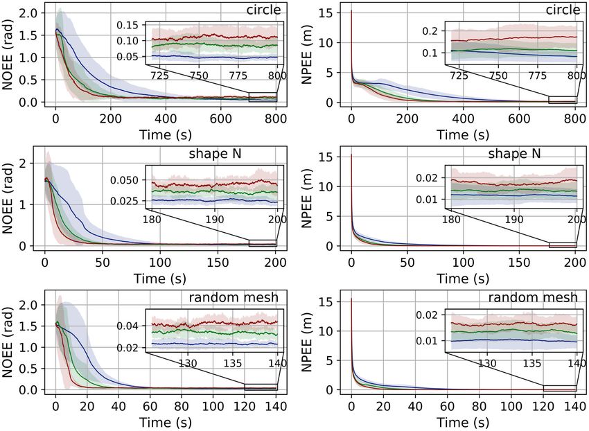
6768                                                                                     IEEE ROBOTICS AND AUTOMATION LETTERS, VOL. 6, NO. 4, OCTOBER 2021

Fig. 3. (Left) Physical postion of agents: each disk represents an agent, the
number on the disk indicates the agent’s id, the dotted line connecting two agents
indicates that those two agents are located within each other’s communication
range. (Right) The horizontal colored arrow lines are agents’ local clocks
running from the left to the right. Each vertical dotted arrow line is a broadcast
event, which points from the transmitter to the receiver(s). Each filled box is a
transmitted message, the box’s color shows its transmitter. The array of unfilled
boxes attached to agent 0’s clock on the bottom shows the values of agent
0’s variable msg_buff at different times t0 , . . ., t5 , each filled box inside the
msg_buff is a received message currently stored in agent 0’s buffer msg_buff.

transmitted message will allow the agent 1 to obtain its own
bearing angle measured by agent 0. Right after transmitting the                                                k
                                                                                          Proposition 1: Let θix     k
                                                                                                                 , θiy  , xki , yik be agent ai ’s pose estimate
message, agent 0 will empty its buffer msg_buff. The agent 0’s
behaviors at t3 , t4 and t5 are almost the same as t0 , t1 and t2 ,                    observed by the global observer at time k f1 , the swarm’s behav-
except that at t5 , it forges the message using the message from                       ior can be described by the Algorithm 2 without loss of any
agent 2 instead of the message from agent 1.                                           information.
   As we discussed before, in the algorithm, each agent ai uses                           Proof: Please see [2], Section VII.
the messages in the buffer msg_buff to update its pose estimate                           Note that the objective fo and fp are defined using the true
at a fixed frequency of f (Algorithm 1, Line 9-29). To do so,                          inter-agent relative bearing angles and distances, whereas in
every f1 amount of time, each agent ai will first uniformly and                        reality, the actual measurements that each agent uses to update
randomly select a message in the buffer msg_buff, which is                             its pose estimate will be corrupted by the sensing noise. Next,
denoted as msg_selected in the algorithm, then, it will check                          we show how the sensing noise and the communication loss will
if the value of the field echo_id in msg_selected matches its                          affect the swarm’s behavior.
                                                                                                                          k
own id, i.e., if this msg_selected contains ai ’s bearing angle                           Lemma 1: Let Θki = [θix  k
                                                                                                                      , θiy  ] be agent ai ’s orientation esti-
                                                                                                                                ∂fo  k
measured by the other. If so, ai will use the information in                           mate at k th iteration, in addition, let ∂Θ   be the value of partial
                                                                                                                                   i
msg_selected to update its pose estimate (Algorithm 1, Line                            derivative of objective fo with respect to Θi calculated using
16-26) and then empty the buffer msg_buff (Algorithm 1, Line                           agents’ orientation estimates at k th iteration, we have:
29). Otherwise, ai will do nothing but empty the buffer msg_buff
directly (Algorithm 1, Line 29). Each time when agent ai updates                                                                  ∂fo k
                                                                                                   E(Θi − Θi ) = −μα
                                                                                                         k+1       k
                                                                                                                                        + γΘk
its pose estimate (Algorithm 1, Line 25-26), the step size is                                                                    ∂Θi
controlled by the variables α and β.
                                                                                       In which:
                                                                                           μ = 1 − (1 − λ)|Ni |                                             (1)
                       IV. THEORETICAL RESULTS
                                                                                                   1 − exp −σ 2 {1 − (1 − λ)|Nj | }
  In this section, we study how each agent’s sensing noise and                            k
                                                                                         γΘ =                 B
                                                                                                                                     R(−Wij )Θkj
communication loss will affect the swarm’s behavior, and we                                                      |Nj |
                                                                                                 aj ∈Ni
show that when the agent’s communication loss and sensing
noise is low, the swarm’s behavior can be approximated as the                                                                        (1 − λ)|Nj | k
unbiased stochastic gradient descent (SGD) on the objective                                                                      −               Θi         (2)
                                                                                                                                        |Nj |
fo and fp . In addition, we give analysis of the algorithm’s
complexity.                                                                                            cos(·), − sin(·)
                                                                                       where R(·) =                         is the rotation matrix con-
                                                                                                        sin(·),    cos(·)
A. Analysis of the Swarm’s Behavior                                                    structed from the angle ·
                                                                                          Proof: Please see [2], Section VIII.
   First, we consider the swarm’s behavior from a global ob-                              Lemma 2: Assume the agents’ orientation estimates have
server’s perspective. Say there is a global observer holding a                         converged to a stable state. Let Xik = [xki , yik ] be agent ai ’s
clock that has the same frequency as each agent’s local clock.                                                                              ∂f k
This global observer will record every agent’s pose estimate at a                      position estimate at k th iteration, moreover, let ∂Xpi be the value
fixed frequency f , which is the same as the frequency at which                        of partial derivative of objective fp with respect to Xi calculated
each agent will attempt to update its pose estimate. By doing                          using agents’ position estimates at k th iteration, we have:
so, this global observer will be able to capture all the changes
                                                                                                                                 ∂fp k
of each agent’s pose estimate. Please see [2] Section VII for the                                  E(Xi  k+1
                                                                                                             − Xi ) = −μβ
                                                                                                                   k
                                                                                                                                        + γXk
formal proof of this conclusion.                                                                                                ∂Xi

          Authorized licensed use limited to: Northwestern University. Downloaded on July 28,2021 at 21:03:10 UTC from IEEE Xplore. Restrictions apply.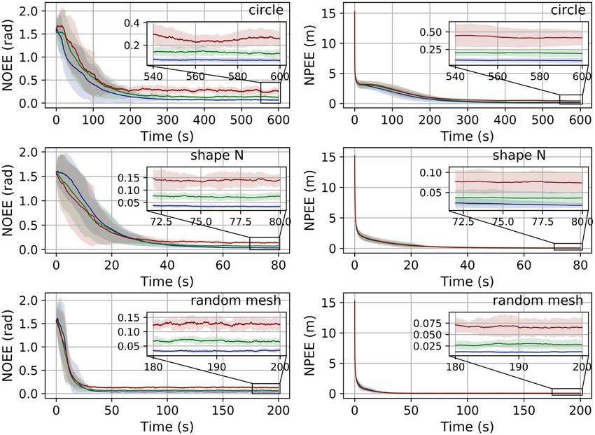
WANG AND RUBENSTEIN: DECENTRALIZED LOCALIZATION IN HOMOGENEOUS SWARMS CONSIDERING REAL-WORLD NON-IDEALITIES                                                  6769

In which:                                                                       B. Complexity
                      |Ni |
   μ = 1 − (1 − λ)                                                       (3)       First, we study the algorithm’s memory complexity. It is
                                σB2
                                                                                straight forward to examine that the memory to execute the
           1 − exp −                {1 − (1 − λ)|Nj | }                        algorithm is dominated by the size of buffer msg_buff. Therefore,
                                 2
 γXk =                                                   P(i, j)dij             for an agent ai , the algorithm’s memory complexity is O(|Ni |),
                                   2|Nj |
         aj ∈Ni
                                                                                where |Ni | is the number of ai ’s neighbors.
                                      (1 − λ)|Nj |                                 Next, we investigate the algorithm’s computation complexity.
                                       +           {Xjk − Xik } (4)             We assume that the complexity of querying a random number
                                         |Nj |                                  generator is O(1), then, the cost to execute Algorithm 1 Line

                       cos(Bij + θi ) − cos(Bji + θj )                          8-32 is O(1). In addition, during a unit of time, each agent ai
where P(i, j) = −                                          is the ma-           can receive at most f |Ni | messages, that is, in a unit of time,
                       sin(Bij + θi ) − sin(Bji + θj )
trix constructed from a pair of agents ai and aj ’s relative bearing            ai will execute Algorithm Line 8-32 at most f |Ni | times. Thus,
angles as well as their orientation estimates.                                  for an agent ai , the computation complexity of the algorithm is
   Proof: Please see [2], Section IX.                                          O(f |Ni |).
   Lemma 1 and Lemma 2 suggest that at each iteration, in                          Lastly, given the fact that the length of each message ex-
expectation, each agent will update its pose estimate along a                   changed amongst the agents is O(1), one can easily conclude
direction that is slightly deviated from the negative gradient of               that the algorithm’s communication complexity, i.e., the amount
objective fp and fo , with a step size that is slightly smaller than            of data to be transmitted by each agent in a unit of time, is O(f ).
the user-specified one. As we can see in Lemma 1 and Lemma
2, the depreciation factor of the step size μ is introduced by                                         V. EMPIRICAL EVALUATION
the agent’s communication loss, in other words, in expectation,                    In this section, we study the performance of proposed algo-
the communication loss will “shorten” the agent’s step size. In                 rithm empirically in a 100-robot swarm and in simulation.
addition, the communication loss’ effect will be reduced by                        To qualitatively evaluate the algorithm’s performance, we
the agent’s degree. As to γΘ and γX (which are the deviation                    introduce two metrics NOEE (normalized orientation estimate
of the expected update direction from the objective’s gradient                  error) and NPEE (normalized position estimate error), which
negative), according to the 2 and 4, they are a result of both the              are the metrics to evaluate the error of agents’ orientation
communication loss and the sensing noise.                                       estimates and position estimates, respectively. The NOEE and
   On the other hand, one can observe that, the bias of the update              NPEE are defined as follows: we use θik = atan2(θiy      k     k
                                                                                                                                            , θix ) and
direction, and the depreciation of the step size will super-linearly            [xi , yi ] to denote agent ai ’s orientation estimate and position
                                                                                   k k
decay over agent’s communication loss and sensing noise. This
                                                                                estimate observed by the global observer at k th iteration, in
suggests that, when communication loss and sensing noise are
                                                                                addition, we use θig and [xgi , yig ] to denote agent ai ’s true pose
reasonably small, the update direction bias γΘ , γX , and the
                                                                                in a global coordinate system. At each iteration k, we first
depreciation of the step size μ will become negligible.
                                                                                calculate the rotation and translation that can match the agents’
   Assumption 1: Each agent ai ’s degree |Ni | is not too low and
                                                                                estimated positions and their true positions the best, namely, find
the packet loss rate 1 − λ is not too high s.t. (1 − λ)|Ni | ≈ 0.               θ∗k ∈ (−π, π], tk∗ ∈ R2 that minimize the following objective:
   Assumption 2: The variance of agent’s bearing sensing noise
  2                           σ2                                                            cos(θk ), − sin(θk ) xk                  g 2
                                                                                                                                           x
σB is not too big s.t. exp{− 2B } ≈ 1.                                              min               ∗               ∗      i
                                                                                                                                 + t∗ − gi
                                                                                                                                    k
   Remark: Assumption 1 and 2 are actually pretty mild. One can                                 sin(θk ),     cos(θk )     yk             y
                                                                                          ai ∈A           ∗               ∗        i                i    2
consider a case where the packet loss rate 1 − λ is 10% and the
lowest degree of any agent in the swarm is 2. In this case, (1 −                Then, the NOEE and NPEE at k th iteration are defined as:
λ)|Ni | = 0.01 ≈ 0. For assumption 2, consider a case where each                                     1  k
                                                                                            NOEEk =        |θi + θ∗k − θig 2π |
agent’s bearing sensing noise has a std of 0.3 rad, which is around                                  n
                                                                                                                 ai ∈A
the same as the std of the angle measurements of Bluetooth 5.1
                                   σ2
                                                                                           cos(θ∗k ), − sin(θ∗k ) xki
                                                                                                                               g
                                                                                                                               xi
devices [20]. In this case, exp − 2B = exp{−0.045} ≈ 1.                             k 1
                                                                                NPEE =                              k + t∗ −
                                                                                                                          k
   Theorem 1: If Assumption 1 and 2 hold, then the swarm’s be-                         n      sin(θ∗ ), cos(θ∗ )
                                                                                                   k         k
                                                                                                                    yi         yig 2
                                                                                               ai ∈A
havior can be approximated as the unbiased stochastic gradient
descent on objective fo and fp . Namely:                                        where n is the swarm size. The NOEE is the normalized geodesic
                                                                                distance between agents’ transformed orientation estimates and
                         ∂fo k                          ∂fp k                   their true orientations, and NPEE is the normalized Euclidean
 E(Θk+1
    i   − Θki ) ≈ −α           , E(Xik+1 − Xik ) ≈ −β
                         ∂Θi                            ∂Xi                     distance between agents’ transformed position estimates and
   Proof: Theorem 1 can be easily obtained by substituting                      their true positions.
                                         σ2
(1 − λ)|Ni | with 1 and substituting exp − 2B with equation
                                                                                A. Simulation
1 in 1, equation 2, equation 3, and equation 4.
   So far, we have shown that when communication loss and                          In simulation, the robot’s communication range is set to 0.3 m,
sensing noise is reasonably small, the swarm’s behavior is                      the robot’s communication frequency f is set to 30 Hz. In each
equivalent to the unbiased SGD on the objective fo and fp .                     test, we place the simulated robots in three patterns: the circle,
In other words, in expectation, the algorithm allows the agents                 the shape “N,” and the random mesh. See Fig. 4 for a graphical
to constantly reduce the disagreement between their pose esti-                  illustration of these three patterns. In the circle pattern, n robots
mates and their local measurements, showing the algorithm’s                     are evenly distributed on on a circle. The circle’s radius is made
correctness.                                                                    such that the distance between two adjacent robots is 0.25 m,

         Authorized licensed use limited to: Northwestern University. Downloaded on July 28,2021 at 21:03:10 UTC from IEEE Xplore. Restrictions apply.
6770 IEEE ROBOTICS AND AUTOMATION LETTERS, VOL. 6, NO. 4, OCTOBER 2021
Fig. 4. From left to right: the circle pattern, the shape “N” pattern, and the
random mesh pattern for a swarm of 35 robots. Each dot represents a robot, a
line connecting two robots indicates that those two robots are located within
each other’s communication range.
Fig. 6. Each colored solid line is the mean from 30 trials, and the colored
shade areas show the confidence intervals for a confidence level of two σ. The
color indicates the swarm size used in the experiment: blue – 64; green – 128;
red – 256.
swarm’s pose estimate converging to a state with higher error.
Furthermore, one can see that compared the other two patterns,
sensing error will affect the circle pattern more significantly.
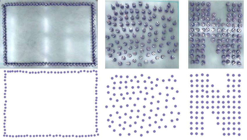
A second test studies the algorithm’s performance on different
Fig. 5. Each colored solid line is the mean from 30 trials, and the colored swarm size. In this test, swarms of 64, 128, 256 robots estimate
shade areas show the confidence intervals at a confidence level of two σ. The their poses with a step size of α = β = 0.2. The communication
color indicates the noise profile used in experiment: blue – σB = 0.05 rad, σd = loss rate 1 − λ is set to 0.1. In addition, the sensing noise is set
0.01 m; green – σB = 0.1 rad, σd = 0.02 m; red – σB = 0.2 rad, σd = 0.04 m.
to σB = 0.05 rad, σd = 0.01 m. For each swarm size, 30 trials
were run. The results are shown in Fig. 6. Unsurprisingly, the
in addition, each robot’s orientation is set to be such that: each results from experiments suggests that for all three patterns, the
agent faces straight towards to the center of the circle. In the swarm size will affect both the convergence rate and the accuracy
shape “N” pattern, the robots’ positions form a “N” shape on of the swarm’s pose estimate: the larger the swarm size is, the
a grid, moreover, the distance between any pair of adjacent slower the swarm’s pose estimate will converge, and the higher
robots is 0.2 m. In the random
√ mesh configuration,
√ n agents are the swarm’s localization error will be.
randomly placed in a 0.25 n m × 0.25 n m space, moreover, In the third test, we study the effect of the step size α and
when generating each robot’s position, we enforce the swarm’s β on the algorithm’s performance. In this test, a swarm of 100
communication graph to be connected. In both shape “N” pat- simulated robots estimate their poses using three different step
tern and random mesh pattern, we set each robot’s orientation sizes: α = β = 0.1, α = β = 0.2, and α = β = 0.3. The com-
randomly. We use these three patterns to investigate the effect munication loss rate 1 − λ is set to 0.1. The noise profile used
of the swarm’s connectivity on the algorithm’s performance. in this test is σB = 0.05 rad, σd = 0.01 m. For each step size, 30
On average, in circle pattern, each agent has 2 neighbors; in trials were run. The results are shown in Fig 7. As we can see in
random mesh pattern, each agent has 4 neighbors; in shape the figure, a larger step size will enable the swarm’s pose estimate
“N” pattern, each agent has 6 neighbors. In all tests, each robot to converge faster, at a cost of swarm’s pose estimate’s accuracy.
ai ’s pose estimate is randomly initialized in a way that x0i ∼ In other words, there is a trade off between the algorithm’s
U (−20, 20), yi0 ∼ U (−20, 20), θi0 ∼ U (−π, π), where U (a, b) convergence rate and localization error. As we can see in the
stands for uniform distribution between the interval (a, b). plots, for all three patterns, the step size α = β = 0.2 seems to
In the first test, we study the effect of sensing noise on the balance the convergence rate and localization error the best.
algorithm’s performance. In this test, a swarm of 100 sim- In the last test, we study the effect of agent’s communication
ulated robots estimate their poses with a step size of α = loss. In this test, a swarm of 100 simulated robots estimate their
β = 0.2. The communication loss rate 1 − λ is set to 0.1. poses with a step size of α = β = 0.2. The noise profile used in
We test the algorithm’s performance with three noise pro- this test is σB = 0.05 rad, σd = 0.01 m. We test the algorithm’s
files: σB = 0.05 rad, σd = 0.01 m; σB = 0.1 rad, σd = 0.02 m; performance with three different communication loss rates:
and σB = 0.2 rad, σd = 0.04 m, where σB , σd are the standard 1 − λ = 0.1, 1 − λ = 0.3, and 1 − λ = 0.5. For each communi-
deviations of robot’s bearing sensing noise and range sensing cation loss rate, 30 trials were run. The results are shown in Fig
noise, respectively. For each noise profile, 30 trials were run. 8. As shown in the figure, unsurprisingly, the communication
The results are shown in Fig 5. As we can see in the figure, for loss will slow down the swarm’s convergence rate. In addition,
all three patterns, the convergence rate of swarm’s pose estimate compared to the other two patterns, the communication loss will
is almost the same for different noise profiles. On the other affect the circle pattern more significantly. The reason is that: in
hand, as expected, the sensing noise will affect the accuracy the circle pattern, the agent’s average degree is much lower than
of the swarm’s pose estimate: bigger sensing noise will result in the other two patterns. This observation confirms our finding in
Authorized licensed use limited to: Northwestern University. Downloaded on July 28,2021 at 21:03:10 UTC from IEEE Xplore. Restrictions apply.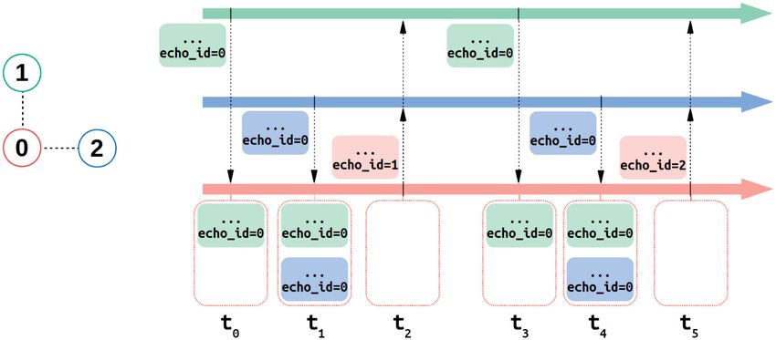
WANG AND RUBENSTEIN: DECENTRALIZED LOCALIZATION IN HOMOGENEOUS SWARMS CONSIDERING REAL-WORLD NON-IDEALITIES                                                  6771

Fig. 7. Each colored solid line is the mean from 30 trials, and the colored         Fig. 9. The solid line is the mean from multiple trials, and the colored shade
shade areas show the confidence intervals for a confidence level of two σ. The      areas show the confidence intervals for a confidence level of two σ.
color indicates the step size used in experiment: blue – α = β = 0.1; green –
α = β = 0.2; red – α = β = 0.3.
                                                                                    B. Experiments
                                                                                       In this section, we examined the algorithm’s performance
                                                                                    on a swarm of 100 Coachbot V2.0 robots [3]. Coachbot V2.0
                                                                                    is a differential driven mobile robot that is able to sense its
                                                                                    position and orientation in a global coordinate system. Note
                                                                                    that Coachbot V2.0 does not have a real bearing and range
                                                                                    sensor. In order to implement our algorithm, in experiments,
                                                                                    we embed the robot’s position in the transmitted data packet,
                                                                                    and the receiver can calculate the transmitter’s bearing and
                                                                                    distance by comparing its own pose with the position contained
                                                                                    in the received message. The limited communication range is
                                                                                    simulated in the same way as [3].
                                                                                       In the experiment, the robot’s communication frequency f is
                                                                                    30 Hz, and the step size is set to α = β = 0.2. The robots are
                                                                                    placed in three patterns: the rectangle pattern, the random mesh
                                                                                    pattern, and the shape “N” pattern. See Fig. 1 for a graphical
                                                                                    illustration of these three patterns. In the rectangle pattern, the
                                                                                    robots are densely placed on the perimeter of a rectangle, where
                                                                                    the distance between two adjacent robots is 0.15 m, and each
Fig. 8. Each colored solid line is the mean from 30 trials, and the colored shade
areas show the confidence intervals for a confidence level of two σ. The color      robot faces straight towards the center of the rectangle. The
indicates the communication loss rate used in experiment: blue – 1 − λ = 0.1;       robot’s communication range is set to 0.2 m in rectangle pattern
green – 1 − λ = 0.3; red – 1 − λ = 0.5.                                             so as to make each robot’s degree to the consistent with the circle
                                                                                    pattern used in the simulation. The remaining two patterns are
                                                                                    the same as the ones used in the simulation, and in those two
                                                                                    patterns, the robot’s communication range is set to 0.3 m. For
Lemma 1 and Lemma 2 that, the effect of communication loss                          the random mesh pattern and the shape “N” pattern, 15 trials
can be reduced by the agent’s degree.                                               were run; for the rectangle pattern, 6 trials were run due to its
   In all four tests, we can see that: compared to the other two pat-               long convergence time. The results are shown in Fig 9.
terns, it takes much longer for the circle pattern to converge. One                    In all the trials, the algorithm reliably converge to all the
possible explanation is that: given n agents, the circle pattern’s                  robots accurately localizing themselves. For each pattern, its
communication diameter, i.e., the maximal pairwise inter-agent                      convergence rate is approximately the same as the result we
communication hop, is O(n), whereas the random mesh pattern    √                    obtained in the simulation. The random mesh pattern and the
and shape “N” pattern has a communication diameter of O( n).                        shape “N” pattern can converge in less than a minute, while
The communication diameter essentially characterizes the cost                       it takes much longer for the rectangle pattern to converge. In
to spread an agent’s information across the entire swarm. The                       addition, one can see that, for random mesh pattern and the
larger the communication diameter is, the longer it will take to                    shape “N” pattern, the average converged NPEE, i.e., normalized
spread a agent’s information across the swarm. As a result, the                     position error, is smaller than 2 cm, and the average converged
larger communication diameter makes circle pattern converge                         NPEE for the rectangle pattern is around 5 cm. Given the fact
much slower than the others. In addition, the difference of each                    that the robot is in a disk shape with a diameter of 13 cm, it
pattern’s communication diameter can also be used to explain the                    can be concluded that, for all three patterns, the robots’ average
observation that the circle pattern has a higher localization error,                converged position error is smaller than the robot’s footprint, and
as the sensing error will accumulate over the communication                         in the case of shape “N” pattern and the random mesh pattern,
hop.                                                                                much smaller.

           Authorized licensed use limited to: Northwestern University. Downloaded on July 28,2021 at 21:03:10 UTC from IEEE Xplore. Restrictions apply.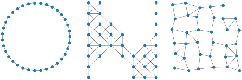
6772                                                                                 IEEE ROBOTICS AND AUTOMATION LETTERS, VOL. 6, NO. 4, OCTOBER 2021

C. Example Use Case: Decentralized Robotic                                          [5] M. Rubenstein and W.-M. Shen, “A scalable and distributed approach for
Shape Formation                                                                         self-assembly and self-healing of a differentiated shape,” in Proc. IEEE
                                                                                        Int. Conf. Robot. Autom., 2008, pp. 1397–1402.
   One desirable feature of our algorithm is that the execution of                  [6] N. K. Long, K. Sammut, D. Sgarioto, M. Garratt, and H. A. Abbass, “A
our algorithm does not require each agent to actively keep the                          comprehensive review of shepherding as a bio-inspired swarm-robotics
                                                                                        guidance approach,” IEEE Trans. Emerg. Topics Comput. Intell., vol. 4,
same neighbors over time, or synchronize its local clock’s phase                        no. 4, pp. 523–537, Aug. 2020.
with the others. This feature makes it possible for the algorithm                   [7] H. Wang and M. Rubenstein, “Walk, stop, count, and swap: Decentralized
to work in the situations where the swarm’s communication                               multi-agent path finding with theoretical guarantees,” IEEE Robot. Autom.
topology is dynamically changing. In this demonstration, 100                            Lett., vol. 5, no. 2, pp. 1119–1126, Apr. 2020.
robots use our algorithm to execute the shape formation algo-                       [8] P. Biswas, T.-C. Lian, T.-C. Wang, and Y. Ye, “Semidefinite programming
                                                                                        based algorithms for sensor network localization,” ACM Trans. Sens.
rithm presented in [3]. Different from the original version of                          Netw., vol. 2, no. 2, pp. 188–220, 2006.
the algorithm presented in [3], where the agents need to acquire                    [9] S. Li, H. Sun, and H. Esmaiel, “Underwater tdoa acoustical location based
their poses from a global position system, in this experiment, the                      on majorization-minimization optimization,” Sensors, vol. 20, no. 16,
robots estimate their poses according to the local measurements                         p. 4457, 2020, doi: 10.3390/s20164457.
                                                                                   [10] M. Imperoli, C. Potena, D. Nardi, G. Grisetti, and A. Pretto, “An effec-
and the odometry. Initially, each robot stays stationary and                            tive multi-cue positioning system for agricultural robotics,” IEEE Robot.
executes our algorithm to estimate its pose. Once the robot’s                           Autom. Lett., vol. 3, no. 4, pp. 3685–3692, Oct. 2018.
pose estimate gets consistent with the local measurements and                      [11] M. L. Elwin, R. A. Freeman, and K. M. Lynch, “Distributed voronoi
its neighbors’ pose estimates, it starts to move to form the                            neighbor identification from inter-robot distances,” IEEE Robot. Autom.
shape. When the robot moves, it uses on-board odometry to                               Lett., vol. 2, no. 3, pp. 1320–1327, Jul. 2017.
                                                                                   [12] M. Rubenstein, A. Cornejo, and R. Nagpal, “Programmable self-assembly
capture the change in its pose over time and updates its pose                           in a thousand-robot swarm,” Science, vol. 345, no. 6198, pp. 795–799,
estimate accordingly, at the same time, it also constantly refines                      2014.
its pose estimate according to the local measurements using our                    [13] J. Klingner, N. Ahmed, and N. Correll, “Fault-tolerant covariance inter-
algorithm. The video of this experiment is shown in [1]. The                            section for localizing robot swarms,” Robot. Auton. Syst., vol. 122, 2019,
                                                                                        Art. no. 103306, doi: 10.1016/j.robot.2019.103306.
result shows that our algorithm successfully enabled the swarm                     [14] D. Moore, J. Leonard, D. Rus, and S. Teller, “Robust distributed network
to replace the use of the global position system with the local                         localization with noisy range measurements,” in Proc. 2nd Int. Conf.
measurements.                                                                           Embedded Networked Sensor Syst., 2004, pp. 50–61.
                                                                                   [15] S. M. Trenkwalder, I. Esnaola, Y. K. Lopes, A. Kolling, and R. Groß,
                                                                                        “Swarmcom: An infra-red-based mobile ad-hoc network for severely
                            VI. CONCLUSION                                              constrained robots,” Auton. Robots, vol. 44, no. 1, pp. 93–114, 2020.
                                                                                   [16] F. K. Chan and H.-C. So, “Accurate distributed range-based positioning
   This letter presents a fully decentralized algorithm for localiz-                    algorithm for wireless sensor networks,” IEEE Trans. Signal Process.,
ing a swarm of identically programmed agents. The execution of                          vol. 57, no. 10, pp. 4100–4105, Oct. 2009.
the presented algorithm does not require each agent to actively                    [17] M. Basiri, F. Schill, P. Lima, and D. Floreano, “On-board relative bearing
keep the same neighbors over time, or synchronize its local                             estimation for teams of drones using sound,” IEEE Robot. Autom. Lett.,
clock’s phase with the others. The theoretical analysis about the                       vol. 1, no. 2, pp. 820–827, Jul. 2016.
                                                                                   [18] A. Cornejo, A. J. Lynch, E. Fudge, S. Bilstein, M. Khabbazian, and
effect of each agent’s sensing noise and communication loss is                          J. McLurkin, “Scale-free coordinates for multi-robot systems with bearing-
given, in addition, the correctness and performance of the algo-                        only sensors,” Int. J. Robot. Res., vol. 32, no. 12, pp. 1459–1474, 2013.
rithm was examined via the tests running on a swarm of up to 256                   [19] J. F. Roberts, T. S. Stirling, J.-C. Zufferey, and D. Floreano, “2.5 d infrared
simulated robots, and 100 real robots. Extensive simulation trials                      range and bearing system for collective robotics,” in Proc. IEEE/RSJ Int.
                                                                                        Conf. Intell. Robots Syst., 2009, pp. 3659–3664.
and real robot experiments show that the algorithm can localize                    [20] M. Cominelli, P. Patras, and F. Gringoli, “Dead on arrival: An empirical
the swarms with different sizes and configurations quickly and                          study of the bluetooth 5.1 positioning system,” in Proc. 13th Int. Workshop
reliably. Furthermore, beyond the situations where the agents are                       Wireless Netw. Testbeds, Experimental Evaluation & Characterization,
stationary, it was shown by a 100-robot experiment that when                            2019, pp. 13–20.
cooperating with the robot’s on-board odometry, the presented                      [21] J. Garcia, S. Soto, A. Sultana, and A. T. Becker, “Localization using a par-
                                                                                        ticle filter and magnetic induction transmissions: Theory and experiments
algorithm can also be used to localize the swarms where the                             in air,” in Proc. IEEE Texas Symp. WMCS, 2020, pp. 1–6.
agents are dynamically moving.                                                     [22] K. Dooley, Designing Large Scale Lans: Help for Network Designers.
                                                                                        “O’Reilly Media, Inc.” 2001.
                                  REFERENCES                                       [23] R. Nagpal, H. Shrobe, and J. Bachrach, “Organizing a global coordinate
                                                                                        system from local information on an Ad Hoc sensor network,” in Inf.
 [1] H. Wang and M. Rubenstein, “Decentralized localization in homogeneous              Process. Sensor Netw.. Springer, 2003, pp. 333–348.
     swarms considering real-world non-idealities (Multimedia Materials),”         [24] R. Spica and P. R. Giordano, “Active decentralized scale estimation for
     2021. [Online]. Available: http://users.eecs.northwestern.edu/~mrubenst/           bearing-based localization,” in Proc. IEEE/RSJ Int. Conf. Intell. Robots
     RAL-IROS-2021.zip                                                                  Syst., 2016, pp. 5084–5091.
 [2] H. Wang and M. Rubenstein, “Decentralized localization in homogeneous         [25] Y. Zou, L. Wang, and Z. Meng, “Distributed localization and circum-
     swarms considering real-world non-idealities (Supplementary Material),”            navigation algorithms for a multiagent system with persistent and inter-
     2021. [Online]. Available: http://users.eecs.northwestern.edu/~mrubenst/           mittent bearing measurements,” IEEE Trans. Automat. Control., 2020,
     supplementary_material_ral2021.pdf                                                 doi: 10.1109/TCST.2020.3032395.
 [3] H. Wang and M. Rubenstein, “Shape formation in homogeneous swarms             [26] Z. Lin, M. Fu, and Y. Diao, “Distributed self localization for relative
     using local task swapping,” IEEE Trans. Robot, vol. 36, no. 3, pp. 597–612,        position sensing networks in 2 d space,” IEEE Trans. Signal Process.,
     Jun. 2020.                                                                         vol. 63, no. 14, pp. 3751–3761, Jul. 2015.
 [4] M. Gauci, R. Nagpal, and M. Rubenstein, “Programmable self-                   [27] L. Carlone and A. Censi, “From angular manifolds to the integer lattice:
     disassembly for shape formation in large-scale robot collectives,” in Proc.        Guaranteed orientation estimation with application to pose graph opti-
     Int. Symp. DARS. Springer, 2018, pp. 573–586, doi: 10.1007/978-3-319-              mization,” IEEE Trans. Robot, vol. 30, no. 2, pp. 475–492, Apr. 2014.
     73008-0_40.

         Authorized licensed use limited to: Northwestern University. Downloaded on July 28,2021 at 21:03:10 UTC from IEEE Xplore. Restrictions apply.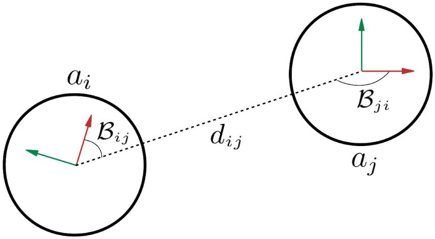
You can also read