Use of Chosen Methods for Determination of the USLE Soil Erodibility Factor on the Example of Loess Slope

Journal of Ecological Engineering Received: 2020.09.10
 Revised: 2020.10.19
Volume 22, Issue 1, January 2021, pages 151–161 Accepted: 2020.11.05
 Available online: 2020.12.01
https://doi.org/10.12911/22998993/128861

Use of Chosen Methods for Determination of the USLE Soil
Erodibility Factor on the Example of Loess Slope

Edyta Kruk1
1
 Department of Land Reclamation and Environmental Development, Faculty of Environmental Engineering
 and Land Surveying, University of Agriculture in Krakow, Al. Mickiewicza 24/28, 30-059 Krakow, Poland
 e-mail: e.kruk@urk.edu.pl

ABSTRACT
The investigations were carried out on a loess slope in the Brzeźnica village, in the Rudnik commune. Nine points
were chosen, in which particular parameters being parts of the examined models, were determined. On the basis
of the literature, eight models for the Universal Soil Loss Equation (USLE) erodibility factor determination were
designated. The chosen models were the ones proposed by: Wishmeier, Monchareonm, Torii et al. and Walker (all
based on texture and organic matter content, Wischmeier and Smith (based on texture organic matter content and
additionally on aggregate classes), Wiliams et al. (based on texture and organic carbon content), Renard et al. as
well as Stone and Hilborn (both based only on texture). The investigated site was characterized as well. The sta-
tistical conclusions were drawn and the obtained results were compared with the results presented in the literature.

Keywords: soil erodibility factor, model USLE

INTRODUCTION along the slope and that there is no plant cover
 for at least two years prior to measurements. For
 Water erosion, along with salinity [Boroń et standard conditions, the coefficients L, S, C and
al. 2010, Boroń et al. 2016, Klatka et al. 2015], P are defined as 1 [Wischmeier and Smith 1978].
drought, floods and heavy metals contamination, Determination of the soil erodibility factor KUSLE
belongs to the most dangerous forms of soil deg- is problematic due to the number of elements
radation. Soil water erosion can be determined in characterizing the soil cover, so various methods
various ways, including modelling, the approach have been developed to quantify it. These meth-
used most often. Among many published soil ods can be divided into direct (field) and indirect
erosion models, Universal Soil Loss Equation approaches (by means of equations and nomo-
(USLE) is the most popular. One of the factors grams). As the field investigations that involve
used in creating this model is the soil erodibility installing measurement systems for effluents on
factor, which depends on the mechanical proper- test plots are costly and time-consuming, they are
ties of the soil. The main factors determining it sometimes impossible to be carried out on a large
are textural properties (granulometry and sorting), scale [Shabani et al. 2014]. In practice, this co-
structural properties (presence of stable soil ag- efficient is therefore calculated by means of em-
gregates), the void ratio and soil moisture [Klatka pirical functions (pedotransfer functions), taking
2020]. The USLE erodibility factor KUSLE express- into account various parameters. Such functions
es the mass of eroded soil (Mg·ha-1) from a stan- describe the relationships between the easily-
dard plot per erodibility unit Je (h·ha-1·MJ-1·cm-1). measurable parameters and the parameters which
A slope of length 22,1 m, width 1.87 m and 9% are more difficult to measure.
inclination was taken as the standard plot in the Wischmeier presented the first method for de-
USLE model [Wischmeier and Smith 1978], as- termining the KUSLE coefficient in 1977 [Torri et
suming that agricultural practices are conducted al. 1997, Ryczek et al. 2013a]. The method was

 151

Journal of Ecological Engineering Vol. 22(1), 2021

based on the 0.1–0.002 mm and < 0.002 mm frac- sand. The KUSLE coefficient was determined by use
tions and organic matter content. Wischmeier and of the Wischmeier and Smith [1978] nomogram.
Smith [1978] introduced a modification of the Święchowicz [2016] investigated the KUSLE factor
equation [Chodak et al. 2008, Ryczek et al. 2013a, in the Łazy village located on the Brzesko Fore-
Panagos et al. 2014] involving water permeabil- land, in the area of the Agricultural Pilot Plant of
ity, structure and the 0.1 – 2 mm fraction. Mon- the Jagiellonian University ‘Łazy’. The texture
chareon (1982) introduced a nomogram [Bahadur was uniform and the sand content was low (be-
2009, Ryczek et al. 2013a], and Williams (1984) low 10%), with high silt content (50–70%) and
discussed the organic matter content [Zhang et al. clay content (8–18%). The organic matter con-
2008]. Modifications were proposed [Renard et tent in the humus horizon was between 0.5 and
al., 1997; Torri et al., 1997] which reduced the in- 1.6%. Relief was characterised by the occurrence
put data only to texture [Drzewiecki and Mularz of curved hilltop hummocks with sections of flat-
2005, Ryczek et al. 2013a, Ryczek et al. 2013b]. tened surfaces, and mainly low-gradient (3–10°)
Stone and Hilborn [2000] used considerable sim- concavo-convex slopes.
plifications concerning the percentage content of Kruk [2016] investigated the soil loss in
organic matter (OM) and soil type. The NRCS the mountain basin of the Mątny stream, which
[2007] elaborated the method, taking into account has an area of 1.47 km2. Soil texture was deter-
the coarse particle content and land use [Ryczek mined for 47 points, with results showing sandy
et al. 2013a]. In 2017, Walker [2017] proposed clay loam, clay loam, loam and silty clay in the
a regression equation that enabled researchers to study area. The author used the Wischmeier and
omit the time-consuming process of determining Smith [1978] and Renard et al. [1997] methods.
KUSLE based on the Wischmeier and Smith nomo- Ryczek et al. [2013b] carried out investigations
gram [1978]. Some investigations [Vaezi et al. in the Smugawka stream basin, located in the Is-
2010] emphasised that KUSLE may be influenced land Beskid region with an area of 5.40 km2. The
by soil structure, and is related to calcium car- KUSLE parameter was determined using the Re-
bonate. In calcareous soil, calcium carbonate in- nard et al. method [1997]. The soils in the basin
fluences the formation of soil aggregates, causing included clay loam, loam, sandy loam and silty
increased water permeability and consequently a clay. The KUSLE factor can also be determined by
decrease in KUSLE [Shabani et al. 2014]. The KUSLE mapping the KUSLE distribution, as elaborated by
values calculated for such soils may not be appro- Panagos et al. [2014], who determined the KUSLE
priate [Vaezi et al. 2010]. based on the Wischmeier and Smith [1978] meth-
 The soil erodibility factor remains the subject od for 25 countries including Poland.
of tests and verifications, so despite the extensive The aim of this work was to compare these
literature on the topic, the best method of calcula- methods for determination of the soil erodibility
tion remains an open question. In Poland, simi- factor, KUSLE, for use in the USLE model.
lar investigations were carried out by Ryczek et
al. [2013a] among others, within the 48.54 km2 Study site
Kasińczanka basin. The authors analysed nine
methods for 52 sampling points located within The study site was an area located in the prov-
the basin, with soil textures including loam, san- ince of Silesia, Racibórz administrative district,
dy clay loam, clay loam and silt loam. The organ- Rudnik commune. The investigated site is geo-
ic matter content was between 1.85 and 4.28%, morphologically part of the Silesia Plain subprov-
while water permeability was between 0.84·10–3 ince, covering all of the western and middle parts
and 4.87·10–1 m·d-1. The following calculation of the Racibórz administrative district in the Oder
methods were used: Wischmeier [1977], Wis- river valley. Two mesoregions occur within the
chmeier and Smith [1978], Monchareon (1982), commune, Głubczyce Plateau and Racibórz Val-
Williams et al. (1984), Renard et al. [1997], Torri ley [Kondracki 2000]. According to the Gumiński
et al. [1997], and Stone and Hilborn [2000] as well agricultural-climatic province categories, the
as the NRCS Kw and the NRCS Kf [2007] mod- area belongs to the Sub Sudety–XVIII province.
els. Baryła [2012] carried out the investigations Masses of wet air from the Atlantic Ocean reach
on the soil mass eroded in the area of the Agri- the area often, with rarer masses of dry continen-
cultural Farm Puczniew (Łódź province). The ar- tal air from the east. Total rainfall is 650 mm per
able lands of the farm consist mostly of loam and year, and there are approximately 40–55 days

152

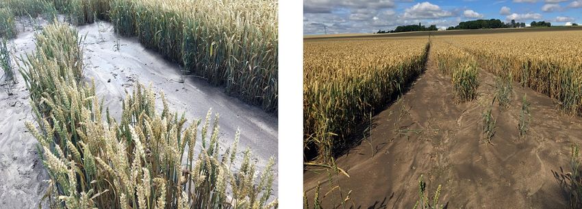
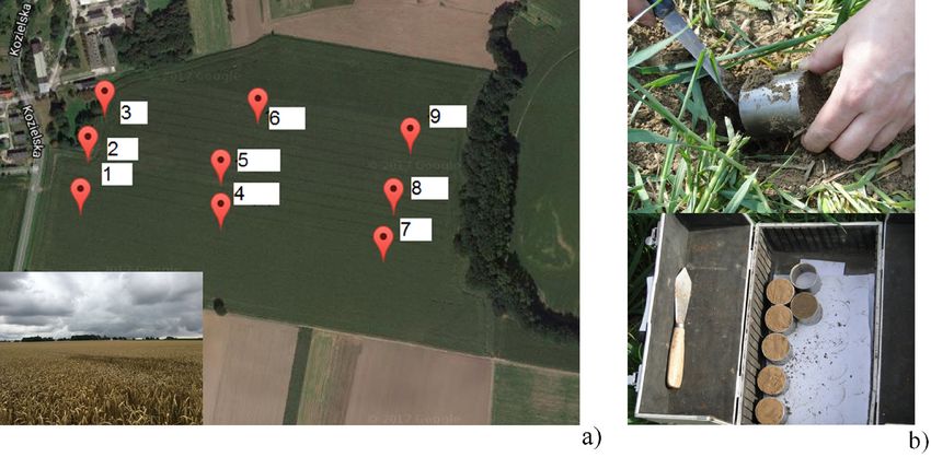
Journal of Ecological Engineering Vol. 22(1), 2021

with snow cover each year. The mean yearly the results were presented in units of Mg·ha·Je-1.
temperature is 8.0°C. The warmest month is July The statistical analyses were performed using the
(mean temperature about 18°C), and lowest tem- Statistica 13.0 software package, using the Least
peratures are recorded in January (mean –2.1°C). Significant Difference (LSD) test and basic sta-
There are typically 30 frosty days and 120 days tistical analysis (Tukey and Fischer-Snedecor
with ground-frost each year. The growing season procedures). The LSD method allowed determin-
starts early, in the second week of March, and ing which differences are statistically significant.
lasts an average of 210­–220 days. Southern and In the case where the absolute value of the dif-
western winds prevail over the area [Radomski ference between the means is greater than LSD
1987, Woś 1993]. The study site was covered by | ̅ − ̅| ≥ , it is assumed that differences
winter wheat during fieldwork on 20 June 2017. are significant. The LSD values were calculated
Before sowing, traditional tillage was used. using the Tukey test, based on the Student t-distri-
 bution. The mathematical model is described as:
Methods xi,j = μ + ρi + τj + εi,j (1)
 Field experimentation was carried out on 20 where: xi,j is the hypothetical value of the investi-
June 2017. Nine measuring points were chosen gated feature of replicate i (i = 1, 2, …..)
(Fig. 1a). Three replicates for each sample were and object j (j = 1, 2, …..),
taken from the upper part of soil, using 100 cm3 μ is the state value estimated by the mean
rings for determination of physical properties of all observations,
(Fig. 1b) and using plastic bags for the remain- ρi is the block component (influence of af-
ing analyses. The following soil properties were filiation to the i-th block),
analysed: texture by means of the Casagrande τj is the object component (influence of
method [PN-R-04032 1998], bulk density (ρo), j-th object),
solid phase density (ρs), total porosity (n) [Mocek εi,j is the random component (error),
et al. 1997, 2015], organic matter content (OM), r is the number of repetitions (blocks),
organic carbon content (C) [Oleksynowa et al. and
1991] and saturated hydraulic conductivity (k) k is the number of factor objects.
[Twardowski and Drożdżak 2006] (Table 1).
 The KUSLE coefficient was calculated using 8 The mean value for each group and object
methods, which depend on various soil proper- mean (from all data), total sum of squares (total
ties. In this work, the models proposed by Wis- variability), total sum of squares between groups
chmeier [1997], Wischmeier and Smith [1978], (from all data) and sum of squares within each
Monchareon (1982) [Bahadur 2009], Williams group (intragroup variability) were determined.
et al. (1984) [Zhang et al. 2008], Renard et al. The F-statistics were then calculated and com-
[1997], Torri et al. [1997], Stone and Hilborn pared with the table values. The results are pre-
[2000] and Walker [2017] (Table 2) were used. All sented in Table 3.

 Figure 1. Location of the points measured in the study site

 153

Journal of Ecological Engineering Vol. 22(1), 2021

Table 1. Soil properties
 Parameter Method
 − 
Bulk density (ρo), Mg·m-3 0 = mmt – dry soil mass with a ring, Mg; mt – mass of a ring,
 
 · 2
 Mg
Internal ring volume (Vp ), m 3 = d – internal ring diameter, m
 4

 – mass of a picnometer with distilled water, Mg
 · . – mass of a picnometer with distilled water and soil,
Solid phase density (ρs), Mg·m -3 =
 + − . Mg
 – water density, Mg∙m-3
 – bulk density, Mg∙m-3,
Total porosity (n), – = 1 −
 – soil phase density, Mg∙m-3,
 The Turin method [Oleksynowa et al. 1991], depending in oxidation of organic mat-
 ter by potassium dichromate (Cr6+).
 Organic matter content was calculated according to the equation:
Organic matter content, (OM), % – amount of 0,2 n FeSO4 for titration of blind sample,
 ( − )∙ ∙0,10344 – 0,2 n FeSO4 ,
 =
 – amount of 0,2 n FeSO4,
 – mass of dry soil

Organic carbon content (C), % % OM = % C ∙ 1,724 1,724 – converting coefficient

Saturated hydraulic conductivity (k), m·d-1 k = C·d102 d10 – diameter of particles, that mass with the mass of
 lower diameter is 10% of sample mass,
Empirical coefficient, C C = 400+40·(n-26) n – total porosity,%

 The total sum of squares (G) was calculated 
according to the equation .. = ∑ ∑ = ∑ = ∑ (8)
 =1 =1 =1 =1
 2 ..2
 = ∑ ∑ , − (2) The sum of squared errors (E) is calculated
 
 =1 =1 according to the equation
 the sum of squares of factors (T) was calcu- E=G–T–R (9)
lated according to the equation LSD was calculated as a product of the stan-
 1
 
 ..2 dard deviation of the means difference sD (based
 2
 = ∑ , − (3) on error due to variance) and the tD–value of the
 dependent variable in relation to significance lev-
 =1
 el α, degrees of freedom for the error (ν) and the
 and the sum of block squares (R) was calcu- number of compared means (m):
lated according to the equation 1
 
 = ( ; , − ) √ [-] (10)
 
 2 ..2
 = ∑ , − (4) where: t(α; k, N – k) is the critical value of the
 
 =1 standardised Student t-test range. The
 standard deviation of the difference be-
 Correction P is calculated according to the tween the means was calculated as:
equation
 2
 2 
 ..2 = √ [-] (11)
 P= (5) 
 
 = ∑ (6)
 =1
 RESULTS AND DISCUSSION
 
 The soil texture was analysed for 9 sam-
 = ∑ (7) ple locations, based on the PN-R-04032
 =1 [1998] standard (table 4). The concentrations

154

Journal of Ecological Engineering Vol. 22(1), 2021

Table 2. Values of the soil erodibility factor KUSLE

 Method Equation

 OM – organic matter content, %, C – content of frac-
Wischmeier [1977], = (12 − ) ∙ [ (100 − )]1,14 tion

Journal of Ecological Engineering Vol. 22(1), 2021

of sand (2.0–0.05 mm), coarse silt (0.05– varied between 2.52 and 2.75 Mg·m-3. OM var-
0.02), fine silt (0.02–0.002 mm) and clay ied from 0.85 to 1.35%, and C fell between 0.52
(

Journal of Ecological Engineering Vol. 22(1), 2021

curves. For sample sites 1, 2, 4, and 6, this value and organic carbon content (C), fell between 0.16
was 82%; for site 3, 80%; for site 5, 81%; for site and 0.18 t·ha-1·Je-1. The values of KUSLE calculat-
7, 83%; for site 8, 86%; and for site 9, 87%. The ed using the Renard et al. method [1997] were
estimated KUSLE values were 0.27–0.31 t·ha-1·Je–1. between 0.41 and 0.43 t·ha-1·Je-1. In the analysis
The values of the 2.0 – 0.1 mm grain size fraction using the Torri et al. equation [1997], calcula-
content for the Wischmeier and Smith method tions were carried out assuming that the lowest
[1978] were 8% for sites 1–3, 5, and 9, 6% for site grain size value of separates is 0.000005 mm;
4, and 7% for sites 6–8. The values of the a param- the results fell between 0.27 and 0.29 t·ha-1·Je-1.
eter were between 0.85 and 1.35%; in all samples For the Stone and Hilborn [2000] method, the
the value of parameter b was found to be 2 (indi- granular subgroups were distinguished based on
cating that aggregates have a fine aggregate struc- the division of mineral deposits into groups and
ture (1 – 2 mm)), and parameter c was found to be subgroups according to PTG [2008], and it was
6 (indicating that the ground has very low perme- found that for all 9 points KUSLE equalled 0,41
ability). The values of the KUSLE parameter were t·ha-1·Je-1. Because of the lack of variability in the
found to be between 0.63 and 0.75 t·ha-1·Je–1. The calculated results, the distribution isolines were
values of KUSLE determined based on the Mon- not generated. During determination of the re-
chareon (1982) method (based on the geometric gression equation for the Walker method [2017],
mean between 3 neighbouring values) were be- 3 random sampling points were chosen (1, 5, 9).
tween 0.55 and 0.57 t·ha-1·Je-1. The KUSLE values This method produced the equation K = 0.0074·S
determined with the Williams method (1984), + 0,0044·C – 0,0925·OM, with KUSLE values rang-
taking into account texture, organic matter (OM) ing between 0.52 and 0.58 t·ha-1·Je-1. According

 Figure 2. Accumulation of soil material dislocated as a result of runoff

Table 6. KUSLE determinations for statistical analysis
 Methods
 A B C D F G H I
 Point Wischmeier Stone
 Wischmeier Monchareonm Wiliams Renard Torii et al. Walker
 and Smith and Hilborn
 [1977] [1982] [1984] et al. [1997] [1997] [2017]
 [1978] [2000]
 1 0.28 0.67 0.55 0.17 0.42 0.28 0.41 0.54
 2 0.27 0.65 0.55 0.17 0.42 0.28 0.41 0.52
 3 0.27 0.63 0.55 0.17 0.42 0.28 0.41 0.53
 4 0.28 0.66 0.56 0.16 0.43 0.29 0.41 0.55
 5 0.28 0.66 0.55 0.17 0.43 0.28 0.41 0.56
 6 0.28 0.65 0.56 0.17 0.43 0.28 0.41 0.53
 7 0.28 0.67 0.56 0.17 0.43 0.29 0.41 0.54
 8 0.31 0.73 0.57 0.17 0.42 0.28 0.41 0.57
 9 0.31 0.75 0.56 0.18 0.41 0.27 0.41 0.58
 Mean 0.28 0.67 0.56 0.17 0.42 0.28 0.41 0.55
 Mean for
 0.42
 methods
 Median 0.41

 157

Journal of Ecological Engineering Vol. 22(1), 2021

to these authors’ suggestion, the KUSLE parameters et al. [1997] (F) and Stone and Hilborn [2000]
for all 9 sampling locations were recorded based (H) methods which make up group c, based on
on the Wischmeier and Smith [1978] method. maximum and minimum grain diameters and
The percentage content of separates with grain their mass share (I), percentage organic mat-
sizes 2–0.1 and 0.1–0.002 mm, and the percent- ter content and soil type information (H). The
age content of organic matter (C) were used in Wischmeier [1977] method (A) and the Torri et
the first approximation. In order to understand al. [1997] method (G), which together compose
variability in the resulting KUSLE values, a second group d and are based on the 0.1–0.002 and <
approximation was made, taking into account soil 0.,002 mm grain size fractions and organic matter
structure and its permeability (Fig. 3). The results content, do not differ statistically from each other.
fell between 0.44 and 0.51 t·ha-1·Je-1 for the first However, they do differ from the other methods.
approximation, and between 0.52 and 0.58 t·ha- Methods F and H both give the values closest
1
 ·Je-1 for the second approximation. The isolines to the mean (0.42 t·ha-1·Je-1) and median values
of spatial distribution for the KUSLE values calcu- (0.41 t·ha-1·Je-1), and thus can be taken as most
lated by these methods are presented in Figure 3. reliable. This study was carried out on a low-in-
The statistical analyses were carried out based on clination slope with uniform soil texture, and the
Table 7, which shows the collected results of the site was covered by uniform plants and consisted
KUSLE calculations, with their mean values and ob- of arable land; it can be therefore assumed that
ject and block sums. disagreement due to random factors was reduced
 The calculated value of the F coefficient to a minimum.
(2880,000) is higher than the value indicated by Comparing the obtained results with the val-
the Fischer-Snedecor distribution tables (2,180), ues from the literature, one can see that Ryczek
which suggests that statistically significant dif- et al. [2013a] obtained the values in the range
ferences exist between all the means. The LSDs 0.072–0.253 Mg·ha·Je-1 using the Wischmeier
between the particular methods were calculated [1977] method; 0.160 – 0.520 Mg·ha·Je-1 using
using the q Tukey test (Table 8). The value of the the Wischmeier and Smith [1978] method; 0.140–
q Tukey parameter, according to the distribution 0.560 Mg·ha·Je-1 using the Monchareon [1982]
tables (at α = 0,05; v = 56; m = 8) is equal to 4.44. method; 0.097–0.196 Mg·ha·Je-1 using the Wil-
LSD is equal to 0.02. liams et al. [1984] method; 0.092–0.439 Mg·ha·Je-1
 From the LSD analysis results, it was found using the Renard et al. [1997] method; 0.091–
that the Wischmeier and Smith [1978] method 0.285 Mg·ha·Je-1 using the Torri et al. [1997]
(B) (group a), based on water permeability, struc- method; and 0.099–0.412 Mg·ha·Je-1 using the
ture and content of the 0.1–2 mm size fraction, Stone and Hilborn [2000] method. Baryła [2012]
differs statistically significantly from the other used the Wischmeier and Smith [1978] method to
methods, as does the Williams (1984) method obtain a KUSLE value of 0.390 t·ha-1·Je-1. Ryczek et
(D) based on the organic matter content method, al. [2013] used the Renard et al. [1997] method for
among other parameters, belonging to group e. the Smugawka stream basin and obtained the val-
The B and D methods should be rejected. The ues of 0.141–0.430 Mg·ha·Je-1 (0.141 Mg·ha·Je-1
Monchareon (1982) method (C), based on the no- for clay loam, 0.430 Mg·ha·Je-1 for silty clay,
mogram with the information on the percentage 0.354 Mg·ha·Je-1 for light loam, 0.279 Mg·ha·Je-1
content of sand, silt and clay separates, and the for sandy clay loam and 0.248 Mg·ha·Je-1 for
Walker [2017] method (I), based on the regres- loam). Święchowicz [2016] obtained a mean
sion equation, make up one group (b) and do not value of 0.377 Mg·ha-1·Je-1 from direct mea-
differ statistically. This is similar to the Renard surements, and a value of 0.738 Mg·ha-1·Je-1 by

Table 7. Analysis of variability F (0.05;7;56)
 Ftab
 Source of variability Degree of freedom Sum of squares Mean squares s2 Fcal
 α=0,05
 Blocks 8 0.01
 Method 7 3.60 0.514286 2880.000 2.180
 Random error 56 0.01 0.000179
 Total 72 1.82

158

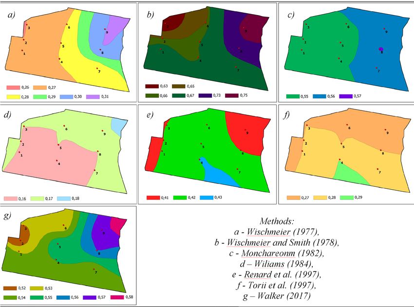
Journal of Ecological Engineering Vol. 22(1), 2021

means of the Wischmeier and Smith [1978] meth- to sandy clay loam and clay loam (0.17 Mg·ha-
od. Kruk [2016] carried out investigations in the 1
 ·Je–1). For loam, the values fall within the range
Mątny stream basin, obtaining the KUSLE values 0.27 – 0.52 Mg·ha-1·Je–1; values > 0.52 Mg·ha-
of 0.14 – 0.57 Mg·ha-1·Je-1 using the Wischmeier 1
 ·Je–1 were obtained mostly from silty clay. Low-
and Smith [1978] method, and the KUSLE values of er values (≤0.41 Mg·ha-1·Je–1) obtained using
0.19 – 0.44 Mg·ha-1·Je-1 using the Renard et al. the second method were mainly from sandy clay
[1997] method. Lower values of KUSLE using the loam and loam. The values > 0.41 Mg·ha-1·Je–1
first method (0.14–0.26 Mg·ha-1·Je–1) were due almost all occurred in silty clay.

 Figure 3. Isolines of the KUSLE distribution calculated according to the following methods: a – Wischmeier,
 b – Wischmeier and Smith, c – Monchareon, d – Williams, e – Renard et al., f – Torri et al., and g – Walker

Table 8. List of means in decreasing order (triangle of differences between means)
 Method Means Triangle of differences between means
 B 0.67
 0.11
 C 0.56 0.12
 0.01 0.25
 I 0.55 0.14 0.26
 0.13 0.15 0.39
 F 0.42 0.14 0.28 0.39
 0.01 0.27 0.28 0.50
 H 0.41 0.14 0.27 0.39
 0.13 0.14 0.38
 A 0.28 0.13 0.25
 0.00 0.24
 G 0.28 0.11
 0.11
 D 0.17
 Means 0.67 0.56 0.55 0.42 0.41 0.28 0.28 0.17
 a
 b b
 c c
 d d
 e

a–e – uniform groups

 159

Journal of Ecological Engineering Vol. 22(1), 2021

 The map of KUSLE factor distributions across & Francis Group London, A Balkema, 245–250.
Europe produced by Panagos et al. [2014], based 5. Chodak T., Tasz W., Kaszubkiewicz J. 2008. An at-
on the Wischmeier and Smith [1978] method, tempt to estimate and verify the USLE model In
shows that the mean KUSLE values for Europe the area of a single slope and agricultural micro-
averaged 0.320 Mg·ha-1·Je-1. The mean val- catchment (in Polish). Materiały Konferencji, Po-
ue for Poland was 0.299 Mg·ha-1·Je-1. For the lanica Zdrój.
Brzeźnica village, this value was between 0.46 6. Drzewiecki W., Mularz S. 2005. Model USPED as
and 0.55 Mg·ha-1·Je-1. a tool for assessment of soil erosion and deposition
 effect) (in Polish). Rocz. Geomat., Tom III, z. 2, 5–9.
 7. Klatka, S. T. 2020. Soil Productivity Index
 in the Selected Area of Post-Mining Geome-
CONCLUSIONS
 chanical Deformations. Journal of Ecologi-
 cal Engineering, 21(5), 148–154. https://doi.
 Different methods of calculating the USLE
 org/10.12911/22998993/122514
soil erodibility factory (KUSLE) produce differing
 8. Klatka S., Malec M., Ryczek M., Boroń K. 2015.
results. The maps of the KUSLE distribution indicate
 Influence of mine activity of the coal mine “Ruch
that this coefficient shows high spatial variability. Borynia” on water management of chosen soils on
The proper determination of the KUSLE coefficient mining area (in Polish). Acta Scientiarum Polono-
is a very real, complicated and important prob- rum Formatio Circumiectus, 14 (1), 115–125.
lem. Detailed statistical analysis of the results 9. Kruk E. 2016. Determination of the probabilisty of
obtained with various methods showed notice- ravine erosion with the use of selected topographic
able differences between the results calculated parameters of a mountains catchment In the Arc-
by means of the Wischmeier and Smith, and Wil- GIS software (in Polish). In: Szałata Ł., Doskocz J.,
liams methods, and between the Wischmeier, and Kardasz P. (Eds.) Innowacje w polskiej nauce w ob-
Torri et al. methods. The Wischmeier and Smith szarze life science i ochrony środowiska: Przegląd
method gives overly high values, while the Wil- aktualnej tematyki badawczej. Wydawnictwo Nau-
liams, Wischmeier and Torri et al. methods give ka i Biznes, 106–117.
lower values in comparison to other ones. They 10. Kondracki J. 2000. Regional geography of Poland
should be used in limited contexts. The most re- (in Polish). Wydanie drugie poprawione, PWN,
 Warszawa.
liable methods are the ones proposed by Renard
et al., and Stone and Hilborn, because they give 11. Mocek A., Drzymała S., Maszner P. 1997. Genesis
the values that fall within the ranges of mean and analysis and classification of soils (in Polish). Wyd.
 Akademii Rolniczej w Poznaniu.
median values obtained for all the methods.
 12. Mocek A. 2015. Soil science (in Polish). Wydawnic-
 two Naukowe PWN, Warszawa.
 13. NRCS (National Resources Conservation Service).
REFERENCES
 2007. Part 618 – Soil Properties and Qualities. US
1. Bahadur K.C.K. 2009. Mapping soil erosion sus- Department of Agriculture, http://soil.usda.gov/
 ceptibility using remote sensing and GIS: A case technical/handbook/contents/part618.html#55.
 of the Upper Nam Wa Watersched, Nan Province, 14. Oleksynowa K., Tokaj J., Jakubiec J. 1991. Guide
 Thailand. Environmental Geology, 57(3), 695–705 to exercies in soil science and geology (in Polish).
2. Baryła A. 2012. Estimating the loss of soil At differ- Wydawnictwo AR, Kraków.
 ent probabilities of erosive rainfalls – a case study of 15. Panagos P., Meusburger K., Ballabio C., Borrelli P.,
 experimental farm in Puczniew (in Polish). Woda Alewell C. 2014. Soil erodibility in Europe: A high-
 – Środowisko – Obszary Wiejskie, 12, 4(40), 7–16. resolution dataset based on LUCAS. Science of the
3. Boroń K., Klatka S., Ryczek M., Liszka P. 2016. Total Environment 479–480, 189–200.
 The formation of the physical, physico-chemical 16. PN-R-04032. 1998. Soil and mineral soil materi-
 and water properties reclaimed and not reclaimed als – Sampling and determination of the grain size
 sediment reservoir of the former Cracow Soda Plant composition (in Polish).
 “Solvay” (in Polish). Acta Scientiarum Polonorum 17. Polskie Towarzystwo Gleboznawcze. 2008. Clas-
 Formatio Circumiectus, 15(3), 35–43. sification of soil and mineral formation (in Polish).
4. Boroń K., Klatka S., Ryczek M., Zając E. 2010. 18. Radomski C. 1987. Agrometeorology (in Polish).
 Reclamation and cultivation of Cracow soda plant PWN, Warszawa.
 lagoons (in Polish). In: Construction for Sustainable 19. Renard K.G., Foster G.R., Weesies G.A, McCool
 Environment. Sarsby & Meggyes, CRC Press Taylor D.K., Yoder D.C. 1997. Predicting Soil Erosion by

160

Journal of Ecological Engineering Vol. 22(1), 2021

 Water: A Guide to Conservation Planning with the of estimating hydraulic properties of grounds (in
 Revised Universal Soil Loss Equation (RUSLE). Polish). Wiertnictwo Nafta Gaz, 23/1, 477–486.
 Agriculture Handbook, US Department of Agricul- 28. USDA. 1951. Soil Survey Manual U.S. Department
 ture, Washington, DC, 73, pp. 251. of Agriculture Handbook 18. US Department of Ag-
20. Rudnicki F. 1992. Agricultural experimental (in Pol- riculture, Soil Conservation Staff, U.S. Government
 ish). Wydawnictwo ATR, Bydgoszcz, pp. 210. Printing Office, Wash. D.C.
21. Ryczek M., Kruk E., Boroń K., Klatka S., Stabryła 29. 2Walker S.J. 2017. An alternative methods for de-
 J. 2013a. Comparison of methods for determination riving a USLE nomograph K factor equation. 22nd
 of soil erodibility factor (k-usle) on the example International Congress on Modelling and Simula-
 of the Kasińczanka stream basin. Acta Scientiarum tion, Hobart, Tasmania, Australia, 3 to 8 December
 Polonorum Formatio Circumiectus 12, 2, 103–110. 2017, 964–970.
22. Ryczek M., Kruk E., Malec M., Klatka S. 2013b. Es-
 30. Wischmeier W.H. 1977. Soil erodibility by rainfall
 timation of water erosion threat of the Smuga stream
 and runoff. In: Toy T.J. (Ed.) Erosion: Research
 basin in the Beskid Wyspowy. Ochrona Środowiska
 techniques, erodibility and sediment delivery. GEO
 i Zasobów Naturalnych 24, 4, 33–37.
 Abstracts, Lid., Norwich, England, 45–56.
23. Shabani F., Kumar L., Esmaeili A., 2014. Improve-
 ment to the prediction of the USLE K factor, Geo- 31. Wischmeier W.H., Smith D D. 1978. Predicting
 morphology 204, 229–234. Rainfall erosion losses – a guide to conservation
 planning. Supersedes Agriculture Handbook No.
24. Stone R.P., Hilborn D., 2000. Universal soil loss
 282; Washington, 4–11.
 equation (USLE). Ontario: Min. Agricult. Food Ru-
 ral Affairs: 1–9. 32. Woś A. 1993. Climatic regions of Poland In the light
 of the frequency of various weathers types (in Pol-
25. Święchowicz, J. 2016. Susceptibility to water ero-
 sion soils derived from less-like depo sits (Brz- ish). Zeszyty Instytutu Geografii i Przestrzennego
 esko Poreland), Southern Poland (in Polish). In: Zagospodarowania, PAN, 20.
 J. Święchowicz & A. Michno (Eds.), Wybrane 33. Vaezi A.R, Bahrami H.A., Sadeghi S.H.R, Mahdian
 zagadnienia geomorfologii eolicznej: Monogra- M.H. 2010. Spatial Variability of Soil Erodibility
 fia dedykowana dr hab. Bogdanie Izmaiłow w 44. Factor (K) of the USLE in North West of Iran. J.
 rocznicę pracy naukowej. Instytut Geografii i Gos- Agr. Sci. Tech. 12, 241–252.
 podarki Przestrzennej UJ Kraków, pp. 331–366. 34. Zhang C., Liu S., Fang J., Tan K. 2008. Research
26. Torri D., Poesen J., Borselli L. 1997. Predictability on the spatial variability of soil moisture based on
 and uncertainty of the soil erodibility factor using a GIS. The International Federation for Information
 global dataset. Elsevier Science B.V., 7–10. Processing, 258, Computer and Computing Tech-
27. Twardowski K., Drożdżak R. 2006. Indirect methods nologies in Agriculture, 1, 719–727.

 161