Saliency Optimization from Robust Background Detection
←
→
Page content transcription
If your browser does not render page correctly, please read the page content below
Saliency Optimization from Robust Background Detection

        Wangjiang Zhu∗                                Shuang Liang†                                 Yichen Wei, Jian Sun
      Tsinghua University                            Tongji University                               Microsoft Research
 wangjiang88119@gmail.com                     shuangliang@tongji.edu.cn                    {yichenw, jiansun}@microsoft.com

                            Abstract                                        serve two drawbacks. The first is they simply treat all image
                                                                            boundary as background. This is fragile and may fail even
    Recent progresses in salient object detection have ex-                  when the object only slightly touches the boundary. The
ploited the boundary prior, or background information, to                   second is their usage of boundary prior is mostly heuristic.
assist other saliency cues such as contrast, achieving state-               It is unclear how it should be integrated with other cues for
of-the-art results. However, their usage of boundary prior                  saliency computation.
is very simple, fragile, and the integration with other cues                    This work presents new methods to address the above t-
is mostly heuristic. In this work, we present new methods                   wo problems. Our first contribution is a novel and reliable
to address these issues. First, we propose a robust back-                   background measure, called boundary connectivity. Instead
ground measure, called boundary connectivity. It charac-                    of assuming the image boundary is background [8, 29], or
terizes the spatial layout of image regions with respect to                 an image patch is background if it can easily be connect-
image boundaries and is much more robust. It has an intu-                   ed to the image boundary [26], the proposed measure states
itive geometrical interpretation and presents unique benefit-               that an image patch is background only when the region it
s that are absent in previous saliency measures. Second, we                 belongs to is heavily connected to the image boundary. This
propose a principled optimization framework to integrate                    measure is more robust as it characterizes the spatial layout
multiple low level cues, including our background measure,                  of image regions with respect to image boundaries. In fac-
to obtain clean and uniform saliency maps. Our formula-                     t, it has an intuitive geometrical interpretation and thus is
tion is intuitive, efficient and achieves state-of-the-art re-              stable with respect to image content variations. This prop-
sults on several benchmark datasets.                                        erty provides unique benefits that are absent in previously
                                                                            used saliency measures. For instance, boundary connectiv-
                                                                            ity has similar distributions of values across images and are
1. Introduction                                                             directly comparable. It can detect the background at a high
    Recent years have witnessed rapidly increasing interest                 precision with decent recall using a single threshold. It nat-
in salient object detection [2]. It is motivated by the im-                 urally handles purely background images without objects.
portance of saliency detection in applications such as object               Specifically, it can significantly enhance traditional contrast
aware image retargeting [5, 11], image cropping [13] and                    computation. We describe and discuss this in Section 3.
object segmentation [20]. Due to the absence of high lev-                      It is well known that the integration of multiple low lev-
el knowledge, all bottom up methods rely on assumptions                     el cues can produce better results. Yet, this is usually done
about the properties of objects and backgrounds. The most                   in heuristic ways [25, 17, 2, 28], e.g., weighted summation
widely utilized assumption is that appearance contrasts be-                 or multiplication. Our second contribution is a principled
tween objects and their surrounding regions are high. This                  framework that regards saliency estimation as a global op-
is called contrast prior and is used in almost all saliency                 timization problem. The cost function is defined to direct-
methods [25, 19, 22, 6, 16, 14, 17, 26, 28, 8, 9, 29, 3].                   ly achieve the goal of salient object detection: object re-
    Besides contrast prior, several recent approaches [26, 8,               gions are constrained to take high saliency using foreground
29] exploit boundary prior [26], i.e., image boundary re-                   cues; background regions are constrained to take low salien-
gions are mostly backgrounds, to enhance saliency compu-                    cy using the proposed background measure; a smoothness
tation. Such methods achieve state-of-the-art results, sug-                 constraint ensures that the saliency map is uniform on flat
gesting that boundary prior is effective. However, we ob-                   regions. All constraints are in linear form and the opti-
  ∗ This work was done while Wangjiang Zhu was an intern at Microsoft       mal saliency map is solved by efficient least-square opti-
Research Asia.                                                              mization. Our optimization framework combines low level
   † Corresponding author.                                                  cues in an intuitive, straightforward and efficient manner.

                                                                        1
This makes it fundamentally different from complex CR- 3.25 23 / 50
F/MRF optimization methods that combine multiple salien-
cy maps [15, 28], or those adapted from other optimization 2.45 34 / 192
problems [23, 29, 9]. Section 4 describes our optimization
method.
In Section 5, extensive comparisons on several bench- 0.43 3 / 49
mark datasets and superior experimental results verify the
effectiveness of the proposed approach. 2.00 6 / 9
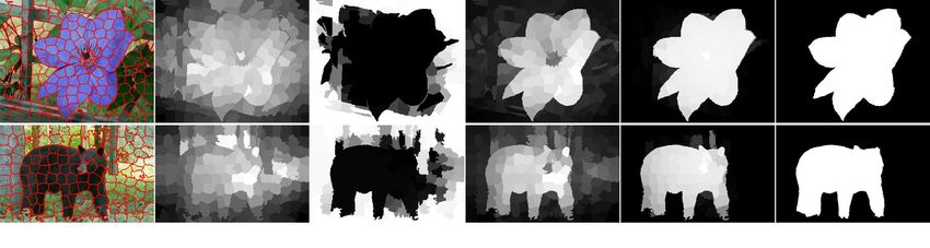
2. Related Work Figure 1. (Better viewed in color) An illustrative example of
boundary connectivity. The synthetic image consists of four re-
Another research direction for visual saliency analy- gions with their boundary connectivity values (Eq.(1)) overlaid.
sis [12, 7, 4, 27, 24, 21] aims to predict human visual at- The boundary connectivity is large for background regions and s-
tention areas. Such works are more inspired by biological mall for object regions.
visual models and are evaluated on sparse human eye fixa-
tion data instead of object/background labelings. We do not of image patches via graph-based manifold ranking. The
discuss such works due to these differences. In the follow- work in [9] models salient region selection as the facility
ing we briefly review previous works from the two view- location problem and maximizes the sub-modular objective
points of interest in this paper: the usage of boundary prior function. These methods adapt viewpoints and optimiza-
and optimization methods for salient object detection. tion techniques from other problems for saliency estima-
Some early works use the so called center prior to bias tion. Unlike all the aforementioned methods, our optimiza-
the image center region with higher saliency. Usually, cen- tion directly integrates low level cues in an intuitive and ef-
ter prior is realized as a gaussian fall-off map. It is either fective manner.
directly combined with other cues as weights [25, 28, 3], or
used as a feature in learning-based methods [24, 8]. This 3. Boundary Connectivity: a Robust Back-
makes strict assumptions about the object size and loca-
ground Measure
tion in the image. From an opposite perspective, recent
works [26, 8, 29] introduce boundary prior and treat image We first derive our new background measure from a con-
boundary regions as background. In [8], the contrast against ceptual perspective and then describe an effective computa-
the image boundary is used as a feature in learning. In [29], tion method. We further discuss the unique benefits origi-
saliency estimation is formulated as a ranking and retrieval nating from its intuitive geometrical interpretation.
problem and the boundary patches are used as background
queries. In [26], an image patch’s saliency is defined as 3.1. Conceptual Definition
the shortest-path distance to the image boundary, observ- We observe that object and background regions in natu-
ing that background regions can easily be connected to the ral images are quite different in their spatial layout, i.e., ob-
image boundary while foreground regions cannot. These ject regions are much less connected to image boundaries
approaches work better for off-center objects but are still than background ones. This is exemplified in Figure 1. The
fragile and can fail even when an object only slightly touch- synthetic image consists of four regions. From human per-
es the boundary1 . In contrast, the proposed new method ception, the green region is clearly a salient object as it is
takes more spatial layout characteristics of background re- large, compact and only slightly touches the image bound-
gions into consideration and is therefore more robust. ary. The blue and white regions are clearly backgrounds as
Most methods implement and combine low level cues they significantly touch the image boundary. Only a small
heuristically. Recently, a few approaches have adopted amount of the pink region touches the image boundary, but
more principled global optimization. In [15], multiple as its size is also small it looks more like a partially cropped
saliency maps from different methods are aggregated into object, and therefore is not salient.
a better one. Similarly, in [28], saliency maps computed on We propose a measure to quantify how heavily a region
multiple scales of image segmentation are combined. These R is connected to the image boundaries, called boundary
methods adopt a complex CRF/MRF formulation and the connectivity. It is defined as
process is usually slow. The work in [23] treats salient ob-
jects as sparse noises and solves a low rank matrix recov- |{p|p ∈ R, p ∈ Bnd}|
BndCon(R) = p (1)
ery problem instead. The work in [29] ranks the similarity |{p|p ∈ R}|
1 A simple “1D-saliency” method is proposed in [26] to alleviate this where Bnd is the set of image boundary patches and p is
problem, but it is highly heuristic and not robust. See [26] for more details. an image patch. It has an intuitive geometrical interpreta-
tion: it is the ratio of a region’s perimeter on the bound-
ary to the region’s overall perimeter, or square root of its
area. Note that we use the square root of the area to achieve
scale-invariance: the measure remains stable across differ-
ent image patch resolutions. As illustrated in Figure 1, the                        (a)                  (b)                 (c)
boundary connectivity is usually large for background re-
gions and small for object regions.                                         Figure 2. (Better viewed in color) Enhancement by connecting im-
                                                                            age boundaries: (a) input image; (b) boundary connectivity with-
3.2. Effective Computation                                                  out linking boundary patches; (c) improved boundary connectivity
    The definition in Eq.(1) is intuitive but difficult to com-             by linking boundary patches.
pute because image segmentation itself is a challenging and
unsolved problem. Using a hard segmentation not only in-
                                                                            where δ(·) is 1 for superpixels on the image boundary and
volves the difficult problem of algorithm/parameter selec-
                                                                            0 otherwise.
tion, but also introduces undesirable discontinuous artifacts
along the region boundaries.                                                    Finally we compute the boundary connectivity in a sim-
    We point out that an accurate hard image segmentation                   ilar spirit as in Eq.(1),
is unnecessary. Instead, we propose a “soft” approach. The
                                                                                                        Lenbnd (p)
image is first abstracted as a set of nearly regular superpix-                              BndCon(p) = p                               (5)
els using the SLIC method [18]. Empirically, we find 200                                                  Area(p)
superpixels are enough for a typical 300∗400 resolution im-
age. Superpixel result examples are shown in Figure 5(a).                       We further add edges between any two boundary super-
    We then construct an undirected weighted graph by con-                  pixels. It enlarges the boundary connectivity values of back-
necting all adjacent superpixels (p, q) and assigning their                 ground regions and has little effect on the object regions.
weight dapp (p, q) as the Euclidean distance between their                  This is useful when a physically connected background re-
average colors in the CIE-Lab color space. The geodesic                     gion is separated due to occlusion of foreground objects, as
distance between any two superpixels dgeo (p, q) is defined                 illustrated in Figure 2.
as the accumulated edge weights along their shortest path                       To compute Eq.(5), the shortest paths between all super-
on the graph                                                                pixel pairs are efficiently calculated using Johnson’s algo-
                                                                            rithm [10] as our graph is very sparse. For 200 superpixels,
                                            n−1
                                            X                               this takes less than 0.05 seconds.
      dgeo (p, q) =         min                   dapp (pi , pi+1 )   (2)
                      p1 =p,p2 ,...,pn =q
                                            i=1
                                                                            3.3. Unique Benefits
   For convenience we define dgeo (p, p) = 0. Then we
define the “spanning area” of each superpixel p as                              The clear geometrical interpretation makes boundary
                                                                            connectivity robust to image appearance variations and sta-
               N                                  N                         ble across different images. To show this, we plot the distri-
               X              d2geo (p, pi )     X
  Area(p) =          exp(−           2       ) =     S(p, pi ), (3)         butions of this measure on four benchmarks on ground truth
               i=1
                                 2σclr           i=1                        object and background regions, respectively, in Figure 3.
where N is the number of superpixels.                                       This clearly shows that the distribution is stable across dif-
    Eq.(3) computes a soft area of the region that p belongs                ferent benchmarks. The objects and backgrounds are clear-
to. To see that, we note the operand S(p, pi ) in the summa-                ly separated. Most background superpixels have values > 1
tion is in (0, 1] and characterizes how much superpixel pi                  and most object superpixels have values close to 0.
contributes to p’s area. When pi and p are in a flat region,                    This property provides unique benefits that are absent in
dgeo (p, pi ) = 0 and S(p, pi ) = 1, ensuring that pi adds a                previous works. As shown in Table 1, when using a sin-
unit area to the area of p. When pi and p are in different                  gle threshold of 2, the proposed measure can detect back-
regions, there exists at least one strong edge (dapp (∗, ∗)                grounds with very high precision and decent recall on all
3σclr ) on their shortest path and S(p, pi ) ≈ 0, ensuring that             datasets. By contrast, previous saliency measures are in-
pi does not contribute to p’s area. Experimentally, we find                 capable of achieving such good uniformity, since they are
that the performance is stable when parameter σclr is within                usually more sensitive to image appearance variations and
[5, 15]. We set σclr = 10 in the experiments.                               vary significantly across images. The absolute value of pre-
    Similarly, we define the length along the boundary as                   vious saliency measures is therefore much less meaningful.
                          N
                                                                                Moreover, an interesting result is that our measure can
                                                                            naturally handle pure background images, while previous
                          X
         Lenbnd (p) =            S(p, pi ) · δ(pi ∈ Bnd)              (4)
                           i=1
                                                                            methods cannot, as exemplified in Figure 4.
1                                0.1    1                                     0.1    1                                   0.1    1                                   0.1
                         object                                       object                                     object                                     object
 0.8                     background 0.08 0.8                          background 0.08 0.8                        background 0.08 0.8                        background 0.08
 0.6                                0.06 0.6                                     0.06 0.6                                   0.06 0.6                                   0.06
 0.4                                   0.04 0.4                                     0.04 0.4                                   0.04 0.4                                   0.04
 0.2                                   0.02 0.2                                     0.02 0.2                                   0.02 0.2                                   0.02
   0                                   0        0                                   0     0                                    0     0                                    0
       0      2        4           6                0      2        4           6              0      2        4           6              0      2        4           6
           Boundary Connectivity                        Boundary Connectivity                      Boundary Connectivity                      Boundary Connectivity

Figure 3. (Better viewed in color) The distribution of boundary connectivity of ground truth object and background regions on four
benchmarks. From left to right: ASD [19], MSRA [25], SED1 [1] and SED2 [1]. Note that we use different y-axis scales for object
and background for better visualization.

                  Boundary Connectivity      Geodesic Saliency
 Benchmark
                  Precision      Recall     Precision      Recall
   ASD [19]         99.7%       80.7%        99.7%        57.4%
  MSRA [25]         98.3%       77.3%        98.3%        63.6%
   SED1 [1]         97.4%       81.4%        96.5%        69.6%
   SED2 [1]         95.8%       88.4%        94.7%        65.7%                                         (a)                        (b)                       (c)
Table 1. Background precision/recall for superpixels with bound-                               Figure 4. (Better viewed in color) A pure background image case.
ary connectivity > 2 on four benchmarks. For comparison, we                                    (a) input image. (b) result of one of the state-of-the-art method-
treat geodesic saliency [26] as a background measure and show its                              s [29]. It is hard to tell whether the detected salient regions are
recall at the same precision. Note, on SED1 and SED2, we cannot                                really salient. (c) boundary connectivity, clearly suggesting that
obtain the same high precision, so the max precision is given.                                 there is no object as all values > 2.

Background Weighted Contrast This highly reliable                                                 According to Eq.(8), the object regions receive high wibg
background measure provides useful information for salien-                                     from the background regions and their contrast is enhanced.
cy estimation. Specifically, we show that it can greatly en-                                   On the contrary, the background regions receive small wibg
hance the traditional contrast computation.                                                    from the object regions and the contrast is attenuated. This
   Many works use the region contrast against its surround-                                    asymmetrical behavior effectively enlarges the contrast dif-
ings as a saliency cue, which is computed as the summation                                     ference between the object and background regions. Such
of its appearance distance to all other regions, weighted by                                   improvement is clearly observed in Figure 5. The original
their spatial distances [22, 16, 17, 28]. In this fashion, a                                   contrast map (Eq.(6) and Figure 5(b)) is messy due to com-
superpixel’s contrast in our notation can be written as                                        plex backgrounds. With the background probability map
                             N
                             X                                                                 as weights (Figure 5(c)), the enhanced contrast map clearly
               Ctr(p) =             dapp (p, pi )wspa (p, pi )                  (6)            separates the object from the background (Figure 5(d)). We
                             i=1                                                               point out that, this is only possible with our highly reliable
                                           d2   (p,pi )
                                                                                               background detection.
where wspa (p, pi ) = exp(− spa    2
                                 2σspa   ). dspa (p, pi ) is the                                  The background probability in Eq.(7) and the enhanced
distance between the centers of superpixel p and pi , and                                      contrast in Eq.(8) are complementary as they characterize
σspa = 0.25 as in [17].                                                                        the background and the object regions, respectively. Yet,
    We extend Eq. (6) by introducing a background proba-                                       both are still bumpy and noisy. In the next section, we
bility wibg as a new weighting term. The probability wibg is                                   present a principled framework to integrate these measures
mapped from the boundary connectivity value of superpixel                                      and generate the final clean saliency map, as in Figure 5(e).
pi . It is close to 1 when boundary connectivity is large, and
close to 0 when it is small. The definition is                                                 4. Saliency Optimization
                                    BndCon2 (pi )
                 wibg   = 1 − exp(−    2          )                             (7)                To combine multiple saliency cues or measures, previ-
                                     2σbndCon
                                                                                               ous works simply use weighted summation or multiplica-
We empirically set σbndCon = 1. Our results are insensitive                                    tion. This is heuristic and hard for generalization. Also, al-
to this parameter when σbndCon ∈ [0.5, 2.5].                                                   though the ideal output of salient object detection is a clean
    The enhanced contrast, called background weighted con-                                     binary object/background segmentation, such as the widely
trast, is defined as                                                                           used ground truth in performance evaluation, most previous
                            N
                                                                                               methods were not explicitly developed towards this goal.
                                   dapp (p, pi )wspa (p, pi )wibg                                  In this work, we propose a principled framework that in-
                            X
           wCtr(p) =                                                            (8)
                            i=1
                                                                                               tuitively integrates low level cues and directly aims for this
(a)                           (b)                          (c)                    (d)                  (e)                   (f)

Figure 5. The pipeline of our method. (a) input images with superpixel boundaries overlaid. (b) contrast maps using Eq.(6). Note that
certain background regions have higher contrast than object regions. (c) background probability weight in Eq.(7); (d) background weighted
contrast using Eq.(8). The object regions are more highlighted. (e) optimized saliency maps by minimizing Eq.(9). (f) ground truth.

goal. We model the salient object detection problem as the                             It is large in flat regions and small at region boundaries.
optimization of the saliency values of all image superpix-                             Note that σclr is defined in Eq.(3). The parameter µ is a
els. The objective cost function is designed to assign the                             small constant (empirically set to 0.1) to regularize the op-
object region value 1 and the background region value 0,                               timization in cluttered image regions. It is useful to erase
respectively. The optimal saliency map is then obtained by                             small noise in both background and foreground terms.
minimizing the cost function.                                                              The three terms are all squared errors and the optimal
   Let the saliency values of N superpixels be {si }N
                                                    i=1 . Our                          saliency map is computed by least-square. The optimiza-
cost function is thus defined as                                                       tion takes 3 millisecond for 200 superpixels in our tests.
                                                                                       This is much more efficient than previous CRF/MRF based
   N                  N
                                                                                       optimization methods [25, 15, 28]. Figure 5 shows the op-
         wibg s2i +         wif g (si − 1)2 +
   X                  X                            X
                                                         wij (si − sj )2         (9)   timized results.
   i=1                i=1                          i,j
   |     {z      }    |        {z              }   |         {z             }
    background              foreground                   smoothness                    5. Experiments
    The three terms define costs from different constraints.                              We use the standard benchmark datasets: ASD [19], M-
The background term encourages a superpixel pi with large                              SRA [25], SED1 [1] and SED2 [1]. ASD [19] is widely
background probability wibg (Eq. (7)) to take a small value                            used in almost all methods and is relatively simple. The
si (close to 0). As stated above, wibg is of high accuracy                             other three datasets are more challenging. MSRA [25] con-
derived from our reliable and stable background detection.                             tains many images with complex backgrounds and low con-
    Similarly, the foreground term encourages a superpix-                              trast objects. SED1 and SED2 [1] contain objects of largely
el pi with large foreground probability wif g to take a large                          different sizes and locations. Note that we obtain the pixel-
value si (close to 1). Note that for wif g we can essential-                           wise labeling of the MSRA dataset from [8].
ly use any meaningful saliency measure or a combination                                   For performance evaluation, we use standard precision-
of them. In Figure 8, we compare several state-of-the-art                              recall curves (PR curves). A curve is obtained by normal-
methods as well as the background weighted contrast in E-                              izing the saliency map to [0, 255], generating binary masks
q.(8) as a simple baseline (all normalized to [0, 1] for each                          with a threshold sliding from 0 to 255, and comparing the
image). Surprisingly we found out that although those mea-                             binary masks against the ground truth. The curves are then
sures have very different accuracies, after optimization they                          averaged on each dataset.
all improve significantly, and to a similar accuracy level.                               Although commonly used, PR curves are limited in that
This is due to our proposed background measure and the                                 they only consider whether the object saliency is higher than
optimization framework.                                                                the background saliency. Therefore, we also introduce the
    The last smoothness term encourages continuous salien-                             mean absolute error (MAE) into the evaluation. It is the av-
cy values. For every adjacent superpixel pair (i, j), the                              erage per-pixel difference between the binary ground truth
weight wij is defined as                                                               and the saliency map, normalized to [0, 1]. It directly mea-
                                                                                       sures how close a saliency map is to the ground truth and is
                                    d2app (pi , pj )                                   more meaningful for applications such as object segmenta-
                     wij = exp(−           2         )+µ                        (10)   tion or cropping. This measure is also used in recent meth-
                                        2σclr
0.25                                                                                     0.25

            0.9                                         0.2                                            0.9                                       0.2
Precision

                                                                                           Precision
            0.8                                        0.15                                            0.8                                      0.15

                                                 MAE

                                                                                                                                          MAE
            0.7    BndCon                               0.1                                            0.7    GS                                 0.1
                   Ctr                                                                                        MR
            0.6    wCtr                                0.05                                            0.6                                      0.05
                                                                                                              BndCon
                   wCtr?                                 0                                                    wCtr?                               0
            0.5                                                   on                   ?               0.5                                                           on       ?
                                                                         r     tr     tr                                                               GS                    tr
               0   0.2   0.4     0.6   0.8   1
                                                              Bn
                                                                dC     Ct    wC     wC
                                                                                                          0   0.2   0.4   0.6   0.8   1                     MR   Bn
                                                                                                                                                                   dC      wC
                            Recall                                                                                    Recall

Figure 6. Comparison of PR curves (left) and MAE (right) on AS-                            Figure 7. PR curves (left) and MAE (right) on MSRA-hard dataset.
D [19] dataset. Note that we use wCtr∗ to denote the optimized
version of wCtr using Eq.( 9).                                                                     Method        SF [17]   GS [26]    HS [28] MR [29] SIA [3]             Ours
                                                                                                   Time           0.16      0.21       0.59    0.25    0.09                0.25
                                                                                                   Code           C++      Matlab     C++     Matlab   C++                Matlab
ods [17, 3] and found complementary to PR curves.                                                        Table 2. Comparison of running time (seconds per image)
    We compare with the most recent state-of-the-art
methods, including saliency filter(SF) [17], geodesic
                                                                                           ingful when the simplicity and efficiency of the weighted
saliency(GS-SP, short for GS) [26], soft image abstrac-
                                                                                           contrast is considered.
tion(SIA) [3], hierarchical saliency(HS) [28] and manifold
ranking(MR) [29]. Among these, SF [17] and SIA [3] com-                                       Example results of previous methods (no optimization)
bine low level cues in straightforward ways; GS [26] and M-                                and our optimization using background weighted contrast
R [29] use boundary prior; HS [28] and MR [29] use global                                  are shown in Figure 9.
optimization and are the best algorithms up to now. There                                     Running time In Table 2, we compare average running
are many other methods, and their results are mostly inferior                              time on ASD [19] with other state-of-the-art algorithms
to the aforementioned methods. The code for our algorithm                                  mentioned above. We implement GS [26] and MR [29] on
and other algorithms we implement is all available online.                                 our own, and use the authors’ code for other algorithms. For
    Validation of the proposed approach To verify the ef-                                  GS [26], we use the same superpixel segmentation [18], re-
fectiveness of the proposed boundary connectivity measure                                  sulting smaller time cost as reported in [26].
and saliency optimization, we use the standard dataset AS-
D. Results in Figure 6 show that 1) boundary connectivity                                  6. Conclusions
already achieves decent accuracy2 ; 2) background weighted                                     We present a novel background measure with intuitive
contrast (Eq.(8)) is much better than the traditional one (E-                              and clear geometrical interpretation. Its robustness makes
q.(6)); 3) optimization significantly improves the previous                                it especially useful for high accuracy background detection
two cues. Similar conclusions are also observed on other                                   and saliency estimation. The proposed optimization frame-
datasets but omitted here for brevity.                                                     work effectively and efficiently combines other saliency
    To show the robustness of boundary connectivity, we                                    cues with the proposed background cue, achieving the state-
compare with two methods that also use boundary prior                                      of-the-art results. It can be further generalized to incor-
(GS [26] and MR [29]). We created a subset of 657 images                                   porate more constraints, which we will consider for future
from MSRA [25], called MSRA-hard, where objects touch                                      works on this subject.
the image boundaries. Results in Figure 7 show 1) bound-
ary connectivity already exceeds GS [26]; 2) the optimized
                                                                                           Acknowledgement
result is significantly better than MR [29].
    Integration and comparison with state-of-the-art As                                       This work is supported by The National Science Founda-
mentioned in Section 4, our optimization framework can                                     tion of China (No.61305091), The Fundamental Research
integrate any saliency measure as the foreground term. Fig-                                Funds for the Central Universities (No.2100219038), and
ure 8 reports both PR curves and MAEs for various saliency                                 Shanghai Pujiang Program (No.13PJ1408200).
methods on four datasets, with before and after optimization
compared. Both PR curves and MAEs show that all meth-                                      References
ods are significantly improved to a similar performance lev-
el. The big improvements clearly verify that the proposed                                      [1] S. Alpert, M. Galun, R. Basri, and A. Brandt. Image seg-
                                                                                                   mentation by probabilistic bottom-up aggregation and cue
background measure and optimization is highly effective.
                                                                                                   integration. In CVPR, 2007. 4, 5, 7
Especially, we find that our weighted contrast (Eq.(8)) can
                                                                                               [2] A. Borji, D.N.Sihite, and L.Itti. Salient object detection: A
lead to performances comparable to using other sophisticat-
                                                                                                   benchmark. In ECCV, 2012. 1
ed saliency measures, such as [28, 29]. This is very mean-
                                                                                               [3] M.-M. Cheng, J. Warrell, W.-Y. Lin, S. Zheng, V. Vineet, and
    2 We normalize and inverse the boundary connectivity map and use it as                         N. Crook. Efficient salient region detection with soft image
a saliency map.                                                                                    abstraction. In ICCV, 2013. 1, 2, 6
0.9                                               0.9                                            0.2
Precision

                                                  Precision
            0.8    SF                                         0.8    MR                                     0.15

                                                                                                      MAE
                   SF?                                               MR?
            0.7    GS                                         0.7    SIA                                     0.1
                   GS?                                               SIA?
            0.6    HS                                         0.6    wCtr                                   0.05
                   HS?                                               wCtr?
            0.5                                               0.5                                             0
               0   0.2   0.4   0.6   0.8      1                  0   0.2     0.4   0.6    0.8     1                SF   GS   HS MR SIA wCtr
                           Recall                                              Recall

            0.9                                               0.9                                            0.2
Precision

                                                  Precision

            0.8    SF                                         0.8    MR                                     0.15
                                                                                                      MAE
                   SF?                                               MR?
            0.7    GS                                         0.7    SIA                                     0.1
                   GS?                                               SIA?
            0.6    HS                                         0.6    wCtr                                   0.05
                   HS?                                               wCtr?
            0.5                                               0.5                                             0
               0   0.2   0.4   0.6   0.8      1                  0   0.2     0.4   0.6    0.8     1                SF   GS   HS MR SIA wCtr
                           Recall                                              Recall

Figure 8. PR curves and MAEs of different methods and their optimized version(∗). From top to bottom: ASD [19], MSRA [25], SED1 [1],
and SED2 [1] are tested. The first two columns compare PR curves and the last column directly shows MAE drops from state-of-the-art
methods (x) to their corresponding optimized results (o).

    [4] D.Gao, V.Mahadevan, and N.Vasconcelos. The discriminant                  [10] Johnson and D. B. Efficient algorithms for shortest paths in
        center-surround hypothesis for bottom-up saliency. In NIPS,                   sparse networks. J. ACM, 24(1):1–13, 1977. 3
        2007. 2                                                                  [11] J.Sun and H.Ling. Scale and object aware image retargeting
    [5] Y. Ding, J. Xiao, and J. Yu. Importance filtering for image                   for thumbnail browsing. In ICCV, 2011. 1
        retargeting. In CVPR, 2011. 1                                            [12] L.Itti, C.Koch, and E.Niebur. A model of saliency-based vi-
    [6] D.Klein and S.Frintrop. Center-surround divergence of fea-                    sual attention for rapid scene analysis. IEEE Transactions
        ture statistics for salient object detection. In ICCV, 2011.                  on Pattern Analysis and Machine Intelligence, 20(11):1254–
        1                                                                             1259, 1998. 2
    [7] J.Harel, C.Koch, and P.Perona. Graph-based visual saliency.              [13] L.Marchesotti, C.Cifarelli, and G.Csurka. A framework for
        In NIPS, 2006. 2                                                              visual saliency detection with applications to image thumb-
    [8] H. Jiang, J. Wang, Z. Yuan, Y. Wu, N. Zheng, and S. Li.                       nailing. In ICCV, 2009. 1
        Salient object detection: A discriminative regional feature              [14] L.Wang, J.Xue, N.Zheng, and G.Hua. Automatic salient ob-
        integration approach. In CVPR, 2013. 1, 2, 5                                  ject extraction with contextual cue. In ICCV, 2011. 1
    [9] Z. Jiang and L. S. Davis. Submodular salient region detec-               [15] L. Mai, Y. Niu, and F. Liu. Saliency aggregation: A data-
        tion. In CVPR, 2013. 1, 2                                                     driven approach. In CVPR, 2013. 2, 5
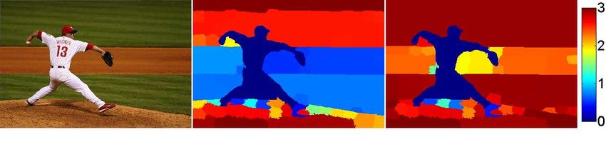
ASD
MSRA
SED1
SED2

       Source image   Ground truth          SF               GS              HS               MR               SIA             wCtr*
                                     Figure 9. Example results of different methods on four datasets.

[16] M.Cheng, G.Zhang, N.Mitra, X.Huang, and S.Hu. Global               [22] S.Goferman, L.manor, and A.Tal. Context-aware saliency
     contrast based salient region detection. In CVPR, 2011. 1, 4            detection. In CVPR, 2010. 1, 4
[17] F. Perazzi, P. Krahenbuhl, Y. Pritch, and A. Hornung. Salien-      [23] X. Shen and Y. Wu. A unified approach to salient object
     cy filters: Contrast based filtering for salient region detec-          detection via low rank matrix recovery. In CVPR, 2012. 2
     tion. In CVPR, 2012. 1, 4, 6                                       [24] T.Judd, K.Ehinger, F.Durand, and A.Torralba. Learning to
[18] R.Achanta, A.Shaji, K.Smith, A.Lucchi, P.Fua, and                       predict where humans look. In ICCV, 2009. 2
     S.Susstrunk. Slic superpixels compared to state-of-the-art         [25] T.Liu, J.Sun, N.Zheng, X.Tang, and H.Shum. Learning to
     superpixel methods. IEEE Transactions on Pattern Analysis               detect a salient object. In CVPR, 2007. 1, 2, 4, 5, 6, 7
     and Machine Intelligence, 34(11):2274–2281, 2012. 3, 6             [26] Y. Wei, F. Wen, W. Zhu, and J. Sun. Geodesic saliency using
[19] R.Achanta, S.Hemami, F.Estrada, and S.Susstrunk.                        background priors. In ECCV, 2012. 1, 2, 4, 6
     Frequency-tuned salient region detection. In CVPR, 2009.           [27] X.Hou and L.Zhang. Saliency detection: A spectral residual
     1, 4, 5, 6, 7                                                           approach. In CVPR, 2007. 2
                                                                        [28] Q. Yan, L. Xu, J. Shi, and J. Jia. Hierarchical saliency detec-
[20] C. Rother, V. Kolmogorov, and A. Blake.                 ”grab-
                                                                             tion. In CVPR, 2013. 1, 2, 4, 5, 6
     cut”cinteractive foreground extraction using iterated graph
     cuts. In SIGGRAPH, 2004. 1                                         [29] C. Yang, L. Zhang, H. Lu, X. Ruan, and M.-H. Yang. Salien-
                                                                             cy detection via graph-based manifold ranking. In CVPR,
[21] R.Valenti, N.Sebe, and T.Gevers. Image saliency by isocen-
                                                                             2013. 1, 2, 4, 6
     tric curvedness and color. In ICCV, 2009. 2
You can also read