Projected incremental changes to extreme wind driven wave heights for the twenty first century
←
→
Page content transcription
If your browser does not render page correctly, please read the page content below
www.nature.com/scientificreports
OPEN Projected incremental changes
to extreme wind‑driven wave
heights for the twenty‑first century
J. G. O’Grady1*, M. A. Hemer2, K. L. McInnes1, C. E. Trenham3 & A. G. Stephenson4
Global climate change will alter wind sea and swell waves, modifying the severity, frequency and
impact of episodic coastal flooding and morphological change. Global-scale estimates of increases
to coastal impacts have been typically attributed to sea level rise and not specifically to changes to
waves on their own. This study provides a reduced complexity method for applying projected extreme
wave changes to local scale impact studies. We use non-stationary extreme value analysis to distil an
incremental change signal in extreme wave heights and associate this with a change in the frequency
of events globally. Extreme wave heights are not projected to increase everywhere. We find that the
largest increases will typically be experienced at higher latitudes, and that there is high ensemble
model agreement on an increase (doubling of events) for the waters south of Australia, the Arabian
Sea and the Gulf of Guinea by the end of the twenty-first century.
Episodic extreme wind-wave events are relevant for probabilistic storm event design studies, to investigate the
capacity of engineered infrastructure or natural environments to withstand the harsh action of the ocean, now
and into the future. Increasing evidence suggests global climate change will alter wind sea and swell waves,
modifying the severity and frequency of episodic coastal flooding and morphological change, exacerbating (or
ameliorating) the impacts of sea level rise (SLR)1.
Coastal flooding studies including the effect of wind waves have attributed global sea level rise with increases
in the frequency of episodic coastal flooding globally using stationary baseline wave climates2–4 and non-station-
ary (baseline and future) wave climates5,6. Vousdoukas et al.5, investigate the influence of SLR combined with
storm surge and wave contribution, but do not specifically detail the contribution of a changing wave climate on
future extreme sea level. Melet et al.7, consider the low-frequency (mean) changes in sea level from the projected
changes in waves. Extreme wave heights on their own are not projected to increase e verywhere8 and the relative
effect of changes to extreme waves rather than SLR on the frequency of coastal impacts has not been shown. The
reduced intensity of episodic extreme wave heights could, for example ameliorate the coastal flooding effect of
SLR, reduce the flushing of stagnate coastal waters9 and/or reduce the depth of closure that relates to the transport
of offshore sediments to the surf zone during episodic events, and therefore sediment availability to replenish
and protect coastlines between storms10.
There is great uncertainty in extreme wave projections due to which future Representative Concentration
Pathway (RCP) will play out as a result of future greenhouse gas emissions, government policies, and technologi-
cal advances11. There is also significant uncertainty in global climate model (GCM) internal accuracy (due to
model resolution and parametrisation) and the significance/robustness of climate statistics, particularly for rare
events (due to limited data in a changing climate). To address the RCP uncertainty, scientific institutions run
GCMs for multiple RCPs to span possible futures, and to address climate sensitivity and model uncertainties mul-
tiple scientific institutions contribute simulations from their own GCMs to projects such as the Coupled Model
Intercomparison project (e.g., CMIP5; CMIP6). The CMIP experiments have enabled the Coordinated Ocean
Wave Climate Project12 to explore robustness and source of uncertainties associated with projected twenty-first
century changes in wind-wave climate, amongst an ensemble of Global Wave Climate Models (GWCM)13,14 .
Extreme value analysis (EVA) provides an avenue to develop extreme value distributions (EVDs) to investigate
the probability of rare and extreme episodic events and how they may change15–17. A three parameter EVD fit is
described by the location, shape and scale parameters, each of which influence the representation of the EVD
and consequently the return level plot (Fig. 1). On the return level curve, with exceedance probabilities plotted
on a logarithmic x-axis, the location parameter describes the vertical offset, the scale parameter is the log-linear
1
CSIRO Oceans and Atmosphere, Melbourne, Victoria, Australia. 2CSIRO Oceans and Atmosphere, Hobart,
Tasmania, Australia. 3CSIRO Oceans and Atmosphere, Canberra, Australian Capital Territory, Australia. 4DATA61
CSIRO, Melbourne, Australia. *email: julian.ogrady@csiro.au
Scientific Reports | (2021) 11:8826 | https://doi.org/10.1038/s41598-021-87358-w 1
Vol.:(0123456789)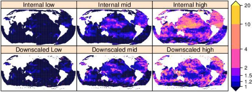
www.nature.com/scientificreports/
Figure 1. Idealised return level diagram describing the EVD location, scale and shape parameters. Red curve is
for a GEV distribution with a positive (+ve) shape parameter typically found at TC latitudes, the black curve is
for a Gumbel distribution (zero shape parameter) and the blue curve is for a GEV distribution with a negative (−
ve) shape parameter typically found at high latitudes. Grey circles represent pseudo empirically-ranked annual
maximum Annual Exceedance Probability (AEP). Created using the R statistical software version 4.0.222.
gradient (slope), and the shape parameter describes the curvature of the return level curve. It has been shown
that at TC locations the shape parameter is positive, and at high latitudes the shape parameter is n egative18.The
shape parameter describes the behaviour of the highest recorded return levels, with larger shape parameters giv-
ing heavier tailed distributions. For a fixed sample size the scale and shape of a distribution is more difficult to
estimate than the location, and therefore robust estimates are more attainable for the location parameter of the
GEV distribution than the scale or shape parameters. Characteristics of projected twenty-first century change
in frequency or intensity of wind-wave events will be represented by changes in these parameters. The shape
parameter is most sensitive to the highest recorded return levels. Thus, robust estimates of the shape parameter
requires many decades of data, and detecting any changes, from a baseline to future climate, requires notionally
twice as much data.
To address statistical significance of rare wave events in a changing climate, different techniques have been
used to gain robustness of extreme estimates. These include non-stationary EVD parameter fitting18–20, methods
for optimal EVD fitting6 and the pooling of multi-model data8. Wind-wave climate EVA could also benefit from
comparing the fit of different EVDs, as has been carried out in studies for extreme sea levels (e.g. Kirezci et al.4;
Wahl et al.21). By their very nature of being rare, a goodness of fit test of empirical data to EVD will always strug-
gle to definitively confirm one modelling technique over another, and therefore model suitability relies on user
and community acceptance of model techniques and assumptions.
Downscaling is a process that brings global scale projections of the future climate to the local scale23,24. The
application, or downscaling, of extreme wave conditions to coastal impact modelling can be resource intensive5,25.
It has been suggested that reduced complexity methods are required to take the globally-resolved simulation of
future wind sea and swell waves to investigate the probabilistic impacts at the local nearshore scale25.
This paper will investigate non-stationary EVD fitting to a global wave hindcast and an ensemble of eight
GWCMs. Using all available GWCM model years, and assuming a non-stationary location parameter (repre-
sentative of climate driven change), we establish single-optimal (stationary) estimates of the scale and shape
parameters (valid over the long-term—towards centennial time-scale) for each GWCM. After demonstrating
that GWCMs are able to replicate the behaviour of the hindcast simulated extreme wave events through EVD
parameters, we introduce a simple reduced complexity change factor (CF) downscaling method. This non-
stationary EVD method presents, for any location, low, mid and high end-ensemble estimates of future wave
heights, as an incremental change relative to baseline extreme wave heights (δHm0).
Results
Extreme value distribution behaviour. We compare the global pattern of both the generalised extreme
value (GEV) EVD, which has a non-zero shape parameter, with the Gumbel EVD which has a shape parameter
of zero, with both fitted to annual maximum v alues15. A hindcast is used as a validation benchmark for an
ensemble of eight global wave models forced with independent GCM surface w inds26. In all EVD modelling a
non-stationary location parameter is used. The EVD modelling makes use of all available years of the 37 year
hindcast and the 66 year GWCMs datasets (i.e. the combination of the 26 year baseline and two 20-year future
time slices for the mid-century and end of century periods) for each of the two different RCPs simulations (RCP
4.5 and RCP 8.5), unless otherwise stated. Results are presented for the low, mid and high-end range of estimates,
represented by the 5th, 50th, and 95th quantiles respectively, to demonstrate the uncertainty range of the bench-
mark hindcast and GWCM ensemble (see “Methods” section).
Scientific Reports | (2021) 11:8826 | https://doi.org/10.1038/s41598-021-87358-w 2
Vol:.(1234567890)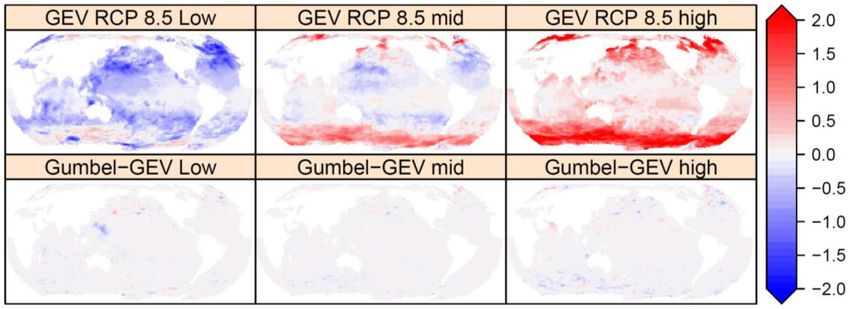
www.nature.com/scientificreports/
Figure 2. Estimated range of the GEV shape parameter for the full periods of the hindcast and GWCM period
(combined baseline, mid and end of twenty-first Century periods) of the two RCP scenarios. Top row: hindcast.
Middle: the entire GWCM RCP 4.5 period. Bottom: same as middle but for RCP 8.5. See "Methods" section for
definition of estimated ranges: low, mid and high represented by the 5th, 50th, and 95th quantiles respectively.
Created using the R statistical software version 4.0.222.
We find that the ensemble range of the EVD parameters fitted to the GWCMs have noticeably similar global
patterns to the span of the benchmark hindcast estimates (Figure 2). This indicates some support for the GWCMs
ability to represent the general nature of extreme wave events given the limitations on GWCM and forcing reso-
lution and physics. Following global satellite a nalysis18, the hindcast and GWCM mid-range estimates indicate:
(1) positive shape parameters at most tropical cyclone (TC) sites, resulting in unbounded annual exceedance
probability (AEP) estimates, and (2) typically negative shape parameters at high latitudes, resulting in bounded
AEP estimates (Figure 2). Overall, the estimates of the shape parameter in the GWCM are lower in magnitude
compared to the hindcast, likely due to the limitations of GWCMs (e.g. grid resolution and parameterised forcing
physics) to fully represent the severity, intensity or occurrence of e xtremes27,28. In Figure 2 we start by focusing on
the GEV shape parameter as it can be considered the most sensitive parameter to the amount of data available,
particularly in a nonstationary c limate19. Figure 2 shows that the two divergent future RCP climate simulations
(RCP4.5 and RCP8.5) have indistinguishable similarity in the shape parameter when considering the unavoidable
spatial variability (noise) due to the sampling of passing storms for the two different simulations. The maximum
likelihood estimate (MLE) GEV shape parameter for each individual GWCM for the RCP 8.5 simulation is shown
in the supplementary report (Figure S1).
Unlike the hindcast, the low end GWCM ensemble estimates indicate that not all models predict a positive
shape parameter at latitudes where TCs occur (Fig. 2). This is consistent with the work of Shimura et al.28, who
found that across this same ensemble of GWCMs, representation of TC driven wave extremes was variable by
model in the Western North Pacific Ocean. Due to the low probability of TC occurrence and underestimated
intensity, future work is required to better represent the intensities of a larger sample of TC extremes, e.g. via
centennial high resolution GWCM or synthetic simulations, to get a better understanding of shape parameter
behaviour28–30.
The high-end GWCM ensemble estimates indicate that not all models, nor all hindcast estimates, indicate
a negative shape parameter at high latitudes (Fig. 2). The hindcast shape parameter in the Southern Ocean
alternates in stripes of positive to negative values across the Southern Ocean. Individual GWCM also show this
striping (Figure S1). We believe this striping is evidence of limited sample of storm tracks in the dataset.
The fitting to the Gumbel EVD shows large scale parameters in the East and South China seas in the hindcast,
which is represented in only a few GWCMs (Figure S2). As with the GEV shape parameter described above,
the two divergent future RCP climate simulations (4.5 and 8.5) have indistinguishable similarity in the Gumbel
scale parameter, suggesting our assumption of a stationary fitting of the scale parameter for a changing climate
is also sensible (Figure S3). It is worth noting here that when the return levels (RL) derived with the Gumbel
distribution are compared to those derived with a strong positive GEV shape parameter (typical of TC locations),
the resulting difference for the 10% AEP RL is small, however for the 1% AEP event the Gumbel EVD has a 40%
lower estimate (Figure S4).
Climate change‑driven alteration of extreme wave heights. Given our assumed stationarity of the
shape and scale parameters, the nonstationary location parameter is used solely to determine the incremental
Scientific Reports | (2021) 11:8826 | https://doi.org/10.1038/s41598-021-87358-w 3
Vol.:(0123456789)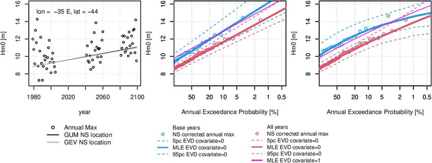
www.nature.com/scientificreports/
Figure 3. Estimated range of the incremental change in extreme wave height (δHm0,100) [m] for the RCP 8.5
simulations over a period of 100 years. Top row GEV RCP 8.5 and bottom row the difference between Gumbel
and GEV RCP 8.5. See "Methods" section for definition of estimated ranges: low, mid and high. Created using
the R statistical software version 4.0.222.
change to future extreme wave climate. Figure 3 shows the centennial (100 year) change in the fitted nonstation-
ary location parameter for the GEV fit (δHm0,100 in metres) to the GWCM ensemble, for the RCP 8.5 scenario,
as described in the “Methods” section. Also shown in Figure 3 are the small differences between the Gumbel and
GEV fits which indicates that the addition of a shape parameter has little influence on detecting the incremental
change in the location parameter.
We find that the parameters of the two EVDs (Gumbel and GEV) fitted independently to either the RCP4.5
or RCP8.5 ensemble simulations have noticeably similar global patterns (Figs. 2, 3 and S3). The only noticeable
difference is that the higher RCP predicts a larger incremental change (positive or negative) in the non-stationary
location parameter (Figure S5). We therefore deduce that changes in extreme wave climate behaviour (storminess
or intensity) in the RCP forced GWCM simulations is not noticeable beyond an incremental change (positive or
negative) to all AEP extremes. The global pattern of incremental change for the two RCP simulations (Figure S5)
show some similarity to the rate of change identified by a linear trend fitted to the annual mean (Figure S6), but
differs in sign at many sites in the North Pacific and Atlantic Oceans, indicating twenty-first century changes in
extreme wave conditions do not necessarily follow the pattern of the mean. The mid-range estimates of δHm0,100
show larger waves at higher latitudes, but also show that subtropical regions could experience a decrease in
extreme wave heights. The high-end estimates indicate that extreme waves (δHm0,100) at high latitude could be
of the order of 2 m taller by the end of the twenty-first century, but not all models predict an increase in extreme
wave heights everywhere. The low-end estimates show that at some sites, even low-end ensemble estimates predict
an increase. The sites showing a high model likelihood of an increase are the waters south-west of Tasmania,
Australia, the Arabian Sea and the Gulf of Guinea.
Figure 4 shows the δHm0 trend in the annual maximum events at a location south of Tasmania, Australia where
there is a high model likelihood/agreement in an increase in future AEPs (Fig. 3). Also shown in Figure 4 are
return level curves (GEV and Gumbel in separate plots) comparing the EVD fitted to 27 year baseline period and
the full GWCM period (66 years over the period 1979 to 2100), i.e. comparing the fully non-stationary fitting of
two time slices, the shape and scale parameters can be different due to sample size. Fitting the GEV distribution
to the baseline periods show a significantly different shape parameter to the full time period, which we believe
is due to sensitivity of fit to record length and not climate change19, as we show the shape parameter is the same
for the two divergent climate scenarios (RCP 4.5 and 8.5; Fig. 2). Further EVD examples for the Arabian Sea and
the Gulf of Guinea and West North Atlantic Ocean are provided in Figure S7.
The incremental change in location parameter δHm0,100 can be easily used in site specific CF downscaling
studies to better identify the future change in the frequency of AEP events (see “Methods” section). The GWCM
EVD parameters can be used to estimate the GWCM internally derived (internal) amplification factor. Alterna-
tively, just the change in the location parameter from a GWCM can be used with hindcast EVA parameters to
estimate the CF “downscaled” amplification. An amplification factor of two implies that what is a 1% AEP (or
1 in 100 year event) in the baseline climate is expected to become a 2% AEP (or 1 in 50 year event) by the end
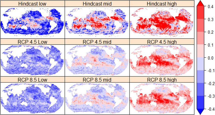
of the twenty-first century. Figure 5 shows the factor of amplification in exceedance probability for the internal
GWCM model GEV parameters, and when δHm0,100 is applied (CF downscaled) to hindcast GEV parameters
(see “Methods” section). Here the differences between the spatial variability in the internally derived GWCM
amplification and the hindcast downscaled are noticeable, where the change in frequency (amplification) of AEP
events is highly sensitive to the spatial variability in the hindcast estimates of EVD shape parameter.
Figure 6 shows the factor of reduction in exceedance probability for the internal GWCM model GEV param-
eters, and when negative δHm0,100 is applied (CF downscaled) to hindcast GEV parameters (see “Methods” sec-
tion). A reduction factor of two implies that what is a 1% AEP (or 1 in 100 year event) in the baseline climate is
expected to become a 0.5% AEP (or 1 in 200 year event) by the end of the twenty-first century. In regions where
there is no amplification (Fig. 5) a reduction is shown. The projected change indicates a decrease in tropical waters
in all oceans, which could potentially result in reduced flushing time of reef lagoons and impact reef h ealth.
Scientific Reports | (2021) 11:8826 | https://doi.org/10.1038/s41598-021-87358-w 4
Vol:.(1234567890)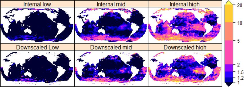
www.nature.com/scientificreports/

                                  Figure 4.  EVD fits to the GFDL-CM3 model output at an example location south of Tasmania, Australia. Left
                                  is time series of annual max Hm0 with the trend line of nonstationary (NS) location parameter for the Gumbel
                                  and GEV fits. Centre plot is Gumbel EVD for the baseline and full RCP85 periods including the MLE and 90%
                                  confidence intervals for the covariate equals zero at 1979 and the MLE for the covariate equals one at 2100.
                                  Right is same as the centre but for a GEV EVD. Created using the R statistical software version 4.0.222.

                                  Figure 5.  GEV RCP85 amplification of the baseline 1% AEP over a period of 100 years. Log colour scale
                                  indicates the amplification factor. Top row: Internal model estimates using GWCM GEV parameters, bottom
                                  row: Downscaled estimates using the hindcast GEV parameters with the incremental change to the location
                                  parameter (δHm0). Created using the R statistical software version 4.0.222.

                                  Figure 6.  Same as Fig. 5 but for a reduction of the baseline 1% AEP over a period of 100 years. created using the
                                  R statistical software version 4.0.222.

Scientific Reports |   (2021) 11:8826 |                https://doi.org/10.1038/s41598-021-87358-w                                                 5

                                                                                                                                             Vol.:(0123456789)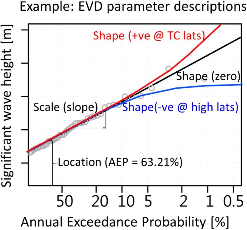
www.nature.com/scientificreports/
Discussion
We show that an ensemble of GWCM forced global wave simulations (GWCMs) spans the range of EVD param-
eters fitted to a detailed hindcast s imulation31,32. The GEV shape parameter, shown to be sensitive to record
length19, along with the Gumbel scale parameter, have indistinguishable similarity in spatial pattern for divergent
RCP simulations (4.5 and 8.5). Thus, an assumption of stationarity in the shape and scale parameters appears
valid for changing climate scenarios. Further consideration should be given to the limitations of a GWCM to
generate intense and random storm climates which could eventuate. The ensemble range of the non-stationary
fit of the location parameter indicates three regions of high model likelihood of an increase. They are the waters
South of Australia, the Arabian Sea, and the Gulf of Guinea. The non-stationary parameter provides an easy to
apply CF downscaling method, e.g. compared to dynamic downscaling, to investigate local coastal impacts of epi-
sodic events. More detailed investigations where the impacts depend on wave direction or period should consider
other more resource-intensive methods, such as dynamic downscaling33,34 or multivariate statistical analysis20,35.
In this study, a limited ensemble of GWCMs that each contain over 60 years of simulation (historical, mid- and
end-Century) were used. Larger ensembles are available that could permit a more complete representation of
uncertainty14. Future studies could broaden the ensemble estimates, provided ensemble members are of sufficient
length to obtain more robust parameter estimates. We present a range of models to allow coastal practitioners to
consider the uncertainty in the modelling estimates, in understanding the ‘worst case’, ‘best case’ and ‘most likely’
GWCM model projection for both an increase and decrease in extreme wave heights in their impact assessment.
GWCMs have shown to exhibit varying levels of bias in the estimate of significant wave height36. In this study,
the method for measuring the change in the location parameter avoids the requirement for bias correction36.
Future work to apply the downscaled changes to coastal impact studies could, for example, revisit investiga-
tions into climate driven changes in the contribution of waves to future extreme sea levels5,37. Due to the low
probability of TC occurrence, future work is required to represent a larger sample of TC extremes, via centennial
GWCM or synthetic simulations, to get a better understanding of shape parameter behaviour. The analysis of
stationary and non-stationary EVD behaviour in GCMs presented here for wind-driven wave heights could also
be considered and tested for other climate variables, such as surface temperatures or wind speeds.
Methods
All model analysis was conducted and plotting/figures created using the R statistical software version 4.0.222.
Global spectral wave model data. Globally gridded annual maximum significant wave heights were
sourced from a hindcast for the period 1979–201832 and eight GWCM ensemble s imulations26. The ¼ nautical
degree hindcast was regridded onto the 1 nautical degree grid of the GWCM using a bilinear point sample, and
all global output projected onto the Robinson projection with the prime meridian centred on the central pacific
dateline38.
Extreme value analysis. Gumbel and GEV extreme value distributions were fitted to annual maximum
significant wave heights using the ‘ismev’ R p ackage15. Nonstationary EVD fitting of the location parameter (µ)
was exclusively applied to all GEV fits in this study. A non-stationary change in the location parameter will there-
fore offset the entire return level curves (Gumbel or GEV) either up or down by a given increment. A covariate
(tc ) representing the temporal change in the EVD location parameter linearly increased from zero in the year
1979 to one in 2100, tc = 2100−1979
nt
, where nt is the number of years to project into the future. The rate of change
in location parameter with the time-covariate ( �t �µ
c
) has units m/year and is used to estimate the incremental
change in extreme significant wave heights (δHm0,nt = �t �µ
c
tc ) with units m over a number of years (nt ). The EVD
fitting was applied to both the annual maxima of baseline period (1979 to 2004) and the full model period of the
hindcast (1979 to 2018) or the GWCMs noncontinuous time slices (baseline spans 1979 to 2004, mid-century
spans 2025 to 2045 and end-of-century spans 2080 to 2100).
The factor of amplification in exceedance probability for the Gumbel EVD was derived f rom39 with the sea
level rise term (δz ) replaced by the incremental change to location parameter (δHm0). GEV factor of increase in
exceedance probability were derived f rom2 with the sea level rise term (µSL) replaced by (δHm0). The factor for the
reduction in exceedance probability is calculated in the same way, except we use the negative of the incremental
change to location parameter (δHm0).
Estimated ranges: low, mid, and high‑end range statistics. We compare the hindcast fitted EVD
uncertainty range to the quantile range of the GWCM model ensemble, both representing 90% range of esti-
mates. Hindcast ranges were derived from plus or minus 1.64 times the standard deviation of EVD fitted param-
eter to represent 90% of EVD fitted uncertainty and the 5, 50 and 95th quantiles. GWCM ranges were calculated
from sample quantiles (5 50 and 95th) of the eight GWCM ensemble using the recommended method of Hynd-
man and Fan40.
Received: 11 December 2020; Accepted: 19 March 2021
Scientific Reports | (2021) 11:8826 | https://doi.org/10.1038/s41598-021-87358-w 6
Vol:.(1234567890)www.nature.com/scientificreports/
References
1. IPCC. Summary for Policymakers. In: IPCC Special Report on the Ocean and Cryosphere in a Changing Climate [H.-O. Pörtner et al].
(2019). http://www.ipcc.ch/publications_and_data/ar4/wg2/en/spm.html.
2. Vitousek, S. et al. Doubling of coastal flooding frequency within decades due to sea-level rise. Sci. Rep. 7, 1–9 (2017).
3. Lambert, E., Rohmer, J., Le Cozannet, G. & Van de Wal, R. S. W. Adaptation time to magnified flood hazards underestimated when
derived from tide gauge records. Environ. Res. Lett. 15, 74015 (2020).
4. Kirezci, E. et al. Projections of global-scale extreme sea levels and resulting episodic coastal flooding over the 21st Century. Sci.
Rep. 10, 1–13 (2020).
5. Vousdoukas, M. I. et al. Global probabilistic projections of extreme sea levels show intensification of coastal flood hazard. Nat.
Commun. 9, 1–12 (2018).
6. Casas-Prat, M. & Wang, X. Projections of extreme ocean waves in the Arctic and potential implications for coastal inundation and
erosion. J. Geophys. Res. Ocean. https://doi.org/10.1029/2019JC015745 (2020).
7. Melet, A. et al. Contribution of wave setup to projected coastal sea level changes. J. Geophys. Res. Ocean. 125, e2020JC0160785
(2020).
8. Meucci, A., Young, I. R., Hemer, M., Kirezci, E. & Ranasinghe, R. Projected 21st century changes in extreme wind-wave events.
Sci. Adv. 6, 1–10 (2020).
9. Taebi, S., et al. Nearshore circulation in a tropical fringing reef system. J. Geophys. Res. 116, C02016 (2011). https://doi.org/10.
1029/2010JC006439.
10. Udo, K., Ranasinghe, R. & Takeda, Y. An assessment of measured and computed depth of closure around Japan. Sci. Rep. 10, 1–8
(2020).
11. van Vuuren, D. P. et al. The representative concentration pathways: An overview. Clim. Change 109, 5–31 (2011).
12. Hemer, M. A., Wang, X. L., Weisssse, R. & Swail, V. R. Advancing wind-waves climate science: The COWCLIP project. Bull. Am.
Meteorol. Soc. 93, 791–796 (2012).
13. Morim, J., Hemer, M. A., Cartwright, N., Strauss, D. & Andutta, F. On the concordance of 21st century wind-wave climate projec-
tions. Glob. Planet. Change 167, 160–171 (2018).
14. Morim, J. et al. Robustness and uncertainties in multivariate wind-wave climate projections. Nat. Clim. Chang. submitted, (2019).
15. Coles, S. An Introduction to Statistical Modeling of Extreme Values. Journal of Chemical Information and Modeling Vol. 53 (Springer,
London, 2001).
16. Gumbel, E. J. The return period of flood flows. Ann. Math. Stat. 12, 163–190 (1941).
17. Jenkinson, A. F. The frequency distribution of the annual maximum (or minimum) values of meteorological elements. Q. J. R.
Meteorol. Soc. 81, 158–171 (1955).
18. Izaguirre, C., Méndez, F. J., Menéndez, M. & Losada, I. J. Global extreme wave height variability based on satellite data. Geophys.
Res. Lett. 38, 1–6 (2011).
19. Vanem, E. Non-stationary extreme value models to account for trends and shifts in the extreme wave climate due to climate change.
Appl. Ocean Res. 52, 201–211 (2015).
20. Davies, G. et al. Improved treatment of non-stationary conditions and uncertainties in probabilistic models of storm wave climate.
Coast. Eng. 127, 1–19 (2017).
21. Wahl, T. et al. Understanding extreme sea levels for broad-scale coastal impact and adaptation analysis. Nat. Commun. 8, 1–12
(2017).
22. R Core Team. R: A Language and Environment for Statistical Computing (R Core Team, 2020).
23. O’Grady, J. et al. Downscaling future longshore sediment transport in south eastern Australia. J. Mar. Sci. Eng. 7, 1–17 (2019).
24. Ekström, M., Grose, M. R. & Whetton, P. H. An appraisal of downscaling methods used in climate change research. Wiley Inter-
discip. Rev. Clim. Chang. 6, 301–319 (2015).
25. Ranasinghe, R. On the need for a new generation of coastal change models for the 21st century. Sci. Rep. 10, 2010 (2020).
26. Hemer, M. A. & Trenham, C. E. Evaluation of a CMIP5 derived dynamical global wind wave climate model ensemble. Ocean Model
103, 190–203 (2016).
27. Timmermans, B., Stone, D., Wehner, M. & Krishnan, H. Impact of tropical cyclones on modeled extreme wind-wave climate.
Geophys. Res. Lett. 44, 1393–1401 (2017).
28. Shimura, T., Mori, N. & Hemer, M. A. Projection of tropical cyclone-generated extreme wave climate based on CMIP5 multi-model
ensemble in the Western North Pacific. Clim. Dyn. 49, 1449–1462 (2017).
29. Bloemendaal, N. et al. Generation of a global synthetic tropical cyclone hazard dataset using STORM. Sci. Data 7, 1–12 (2020).
30. Walsh, K. J. E. et al. Tropical cyclones and climate change. Wiley Interdiscip. Rev. Clim. Chang. 7, 65–89 (2016).
31. Hemer, M. A. et al. A revised assessment of Australia’s national wave energy resource. Renew. Energy 114, 85–107 (2017).
32. Smith, G. A. et al. Global wave hindcast with Australian and Pacific Island Focus: From past to present. Geosci. Data J. https://doi.
org/10.1002/gdj3.104 (2020).
33. Charles, E. et al. Climate change impact on waves in the Bay of Biscay, France. Ocean Dyn. 62, 831–848 (2012).
34. Wandres, M., Pattiaratchi, C. & Hemer, M. A. Projected changes of the southwest Australian wave climate under two atmospheric
greenhouse gas concentration pathways. Ocean Model 117, 70–87 (2017).
35. Antolínez, J. A. A. et al. Downscaling changing coastlines in a changing climate: The hybrid approach. J. Geophys. Res. Earth Surf.
123, 229–251 (2018).
36. Lemos, G. et al. On the need of bias correction methods for wave climate projections. Glob. Planet. Change 186, 103109 (2020).
37. O’Grady, J. G. et al. Extreme water levels for Australian beaches using empirical equations for shoreline wave setup. J. Geophys.
Res. Ocean. 124, 5468–5484 (2019).
38. Hijmans, R. J. et al. Package ‘raster’. Cran 1–249 (2020).
39. Hunter, J. R. Estimating sea-level extremes under conditions of uncertain sea-level rise. Clim. Change 99, 331–350 (2010).
40. Hyndman, R. J. & Fan, Y. Sample quantiles in statistical packages. Am. Stat. 50, 361–365 (1996).
Author contributions
J.G.O and M.A.H conceived the study and designed it with K.L.M and A.G.S jointly. J.G.O performed the analysis
and developed the figures. C.E.T. prepared the datasets. J.G.O. wrote the manuscript. All of the authors contrib-
uted to make substantial improvements to the manuscript.
Funding
This study was supported by the Earth Science and Climate Change Hub of the Australian Government’s National
Environmental Science Programme (NESP).
Competing interests
The authors declare no competing interests.
Scientific Reports | (2021) 11:8826 | https://doi.org/10.1038/s41598-021-87358-w 7
Vol.:(0123456789)www.nature.com/scientificreports/
Additional information
Supplementary Information The online version contains supplementary material available at https://doi.org/
10.1038/s41598-021-87358-w.
Correspondence and requests for materials should be addressed to J.G.O.
Reprints and permissions information is available at www.nature.com/reprints.
Publisher’s note Springer Nature remains neutral with regard to jurisdictional claims in published maps and
institutional affiliations.
Open Access This article is licensed under a Creative Commons Attribution 4.0 International
License, which permits use, sharing, adaptation, distribution and reproduction in any medium or
format, as long as you give appropriate credit to the original author(s) and the source, provide a link to the
Creative Commons licence, and indicate if changes were made. The images or other third party material in this
article are included in the article’s Creative Commons licence, unless indicated otherwise in a credit line to the
material. If material is not included in the article’s Creative Commons licence and your intended use is not
permitted by statutory regulation or exceeds the permitted use, you will need to obtain permission directly from
the copyright holder. To view a copy of this licence, visit http://creativecommons.org/licenses/by/4.0/.
© The Author(s) 2021
Scientific Reports | (2021) 11:8826 | https://doi.org/10.1038/s41598-021-87358-w 8
Vol:.(1234567890)You can also read