Supplement of Surface deformation relating to the 2018 Lake Muir earthquake sequence, southwest Western Australia: new insight into stable ...
←
→
Page content transcription
If your browser does not render page correctly, please read the page content below
Supplement of Solid Earth, 11, 691–717, 2020
https://doi.org/10.5194/se-11-691-2020-supplement
© Author(s) 2020. This work is distributed under
the Creative Commons Attribution 4.0 License.

Supplement of
Surface deformation relating to the 2018 Lake Muir earthquake
sequence, southwest Western Australia: new insight into stable
continental region earthquakes
Dan J. Clark et al.

Correspondence to: Dan J. Clark (dan.clark@ga.gov.au)

The copyright of individual parts of the supplement might differ from the CC BY 4.0 License.
Supplementary information

     UAV DTM processing workflow and DBCA LiDaR details

     In order to recover the surface deformation envelope associated with the events, aerial photographs were acquired with a DJI
 5   Phantom 4 UAV in an approximately 500 m-wide swath along an approximately 2 km length of the scarp produced in the
     September event. A ~2 km-long cross-line was also flown, extending eastward from the scarp across the region of most
     significant surface deformation indicated in the InSAR data (Figure 3). Flights were planned in the Map Pilot software (version
     3.0.0) provided by Drones Made Easy (https://support.dronesmadeeasy.com/hc/en-us/categories/200739936-Map-Pilot-for-
     DJI). The 1144 images were captured in RAW format from an average elevation above the take-off point of 100 m, with 75%
10   overlap in the forward and sideward directions, achieving an effective ground sampling distance of ~5.25 cm. Seventeen
     ground control points (GCPs) were deployed within the 1.75 km2 mission area, and their locations were surveyed to better than
     0.03 m accuracy in the horizontal and 0.06 m accuracy in the vertical using an Altus RTK GPS system. Due to the size of the
     area being captured, the coverage was acquired over two days.
     The image dataset was processed using a Structure-from-Motion (SfM) and multi-view stereo approach, implemented in the
15   software Agisoft Photoscan Pro 1.4.3 (Agisoft LCC). Initial image alignment and production of a sparse point cloud was
     achieved using the approximate 3D position, roll, pitch and yaw of the UAV captured by the UAV’s on-board GPS and an
     inertial measurement unit. The GCPs were then manually identified on the images and their co-ordinates imported. The co-
     ordinates of the GCPs were used to refine the camera calibration parameters, and to optimise the geometry of the sparse point
     cloud. Multi-view stereo image matching algorithms (Seitz et al., 2006), implemented in Agisoft Photoscan Pro 1.4.3, were
20   then applied to densify the sparse point cloud. The resulting dense point cloud achieved a standard deviation of the location
     differences between it and the control points of 0.09 m in the horizontal and 0.01 m in the vertical, which is comparable to
     other studies using similar GCP densities (e.g. Gindraux et al., 2017).          Several studies of factors impacting local
     photogrammetry-derived DSM accuracy (e.g. Tonkin and Midgley, 2016; Gindraux et al., 2017) report a vertical accuracy
     decrease of ~0.1 m for every 100 m increase in the distance to the closest GCP. In extreme cases this can result in a ‘bowl’ or
25   ‘dome’ effect (e.g. Ouédraogo et al., 2014). In our study the maximum distance from a control point is in the order of 200-
     300 m.
     The dense point cloud was exported to the American Society for Photogrammetry and Remote Sensing (ASPRS) LAS format
     and classified into ground and non-ground points using the Cloth Simulation Filtering algorithm (Zhang et al., 2016; Serifoglu
     Yilmaz et al., 2018) implemented in the open source software package CloudCompare (https://www.danielgm.net/cc/). Points
30   comprising the ground class were then re-imported into Photoscan, and a 6 cm-resolution Digital Terrain Model (DTM) was

                                                                   1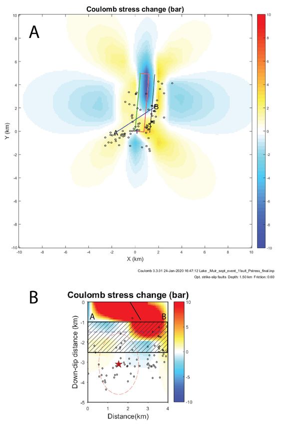
generated. The DTM was used within the software to produce an orthophoto, then exported to geotiff format for further
     analysis.
     In January 2012, the Western Australia Government Department of Biodiversity, Conservation and Attractions (DBCA)
     acquired a 1 m gridded LiDAR DTM covering the study area. The average magnitude of the uncertainties associated with the
35   elevation values for this dataset is reported as 0.063±0.074 m. The elevation values from a subset of the LiDAR were subtracted
     from the ground class DTM generated in this study, to produce a DTM of difference (DoD, Williams, 2012). Voids in the DoD
     were filled using the ESRI ArcGIS focal statistics tool (null values are filled with the mean value within a rectangular
     neighbourhood of 50 cells dimension).
     Change in land use from forestry to pasture in the time between acquisition of the LiDAR and UAV datasets has resulted in
40   the introduction of several artefacts into the differenced DEM. For example, forestry practice involved the construction of
     numerous parallel furrows up to 0.1 – 0.2 m high and at 3 – 4 m spacing, into which pine trees were planted. The relief on
     these furrows has significantly eroded in the 6.5 years between the acquisition of the datasets. Several dams have also been
     constructed, one of which resulted in the modification of a wetland. Despite these sources of ‘cultural noise’, the vertical
     displacement envelope resulting from the September earthquake was able to be recovered from the DoD, with an accuracy of
45   approximately 0.1 - 0.2 m.
     A third UAV mission covered the southern extent of surface deformation indicated in the InSAR imagery (Figures 3, S1). Six
     GCPs were deployed within the 0.86 km2 mission area, and their locations were surveyed to better than 0.02 m accuracy in the
     horizontal and 0.04 m accuracy in the vertical using an Altus RTK GPS system. A DoD was calculated using the same
     methodology above. The DoD shows the faint but continuous trace of a rupture that is everywhere less than 5 cm in height.
50   While this displacement magnitude is consistent with the estimates using the unwrapped InSAR (Figure 6b), the orientation of
     the rupture at this location, sub-parallel to the maximum compression direction of the crustal stress field (Rajabi et al., 2017),
     suggests that horizontal motion may have been dominant. The vertical UAV signature might result in part from horizontal
     displacement of furrows associated with the former forestry land-use.

                                                                     2
55 Figure S1: UAV DoD for the southern terminal structure (see Figure 3 for location). Subtle scarp with
to uncertainties in earth structure along the event-station ray path. The algorithm works by first establishing a network of
     differential P- and S-wave travel times between two proximally located hypocentres that share a minimum number of P- and
70   S-phase arrivals at common stations. This network of events is determined through initial parameterization using the Ph2dt
     program (Table S1). This parameterization includes setting a maximum separation distance in kilometres (MAXSEP), a
     minimum number of phase pairs (MINLNK), and a maximum number of neighbouring events (MAXNGH). To establish
     strong links between events, Waldhauser (2001) recommends at least eight observations (MINOBS) for each event pair. Table
     S1 outlines the initial parameters used in the Ph2dt program for the Lake Muir earthquakes. MAXDIST specifies the distance
75   between the event and station in km, and was set to a default value of 100, which includes all stations capable of recording the
     smaller-magnitude aftershocks in the Lake Muir area. Only events from the original dataset that meet this initial criteria are
     used in the HypoDD inversion. As a result, catalogue P- and S-wave data from 470 events were included in the final relocation.

80   Table S1 Ph2dt input Parameters

     Once events are linked together with the Ph2dt program and networks of event pairs are generated, HypoDD groups these
     events into clusters and then minimizes the travel-time residuals by adjusting the spatial difference of the hypocentres relative
     to the other hypocentres within the cluster. The double-difference travel-time residual is the difference between the observed
85   and theoretical travel times for each event pair. The source of the P- or S-wave travel time differences of two events at one
     station can then be attributed to a spatial offset between the hypocentres, since the ray paths between the earthquake source
     and the seismic station are assumed to be similar. Theoretical travel times are calculated using a 1-D P-wave velocity model,
     which is derived from Dentith et al. (2000) and Salmon et al. (2012) and incorporates a shallow, low-velocity sediment layer.
     The VP/VS ratio was set to 1.73.
90

     Table S2 1-D P-wave velocity model

     The double-difference travel-time residuals are minimized by weighted least squares. The Singular Value Decomposition
95   (SVD) inversion method was chosen as the preferred inversion method, because SVD can examine smaller clusters of events
     and can also produce meaningful three-dimensional hypocentre relocation error estimates (2001). Before running the
     inversion, the original earthquake locations were separated into four different datasets, shown by the dashed boxes in Figure

                                                                    4
1. The events were split to regulate the size of the relocation inversion problems to be solved. The aftershocks in subset A
were restricted to magnitudes ML ≥ 1.0, since the total number of events near the focus of the 16 September mainshock would
100 be too large for the SVD inversion method. This magnitude threshold also ensures that the earthquakes are clearly recorded
by both the local Lake Muir stations and by regional ANSN stations. Subset D was relocated separately, because these
aftershocks temporally relate to the 16 September mainshock and are spatially related to the southern extent of surface rupture.
The number of earthquakes and delay times for each subset A-D are shown in Table S3.
105
Table S3 Earthquake and delay time counts
Within subset A, the A-A’ cross-section is oriented approximately normal to the strike direction of the 16 September, 2018
focal mechanism. These events relocate to depths between 1 and 4 km (Figure S2). There is no clearly defined dip angle to
110 this event cluster. Within subset B and along the B-B’ cross-section, which is normally oriented to the discrete surface rupture,
the earthquakes are also clustered between 1 and 4 km depth. East of the cross-section centre, the aftershocks dip ~30° to the
east. The C-C’ cross-section is oriented NW-SE: normal to the north-east trending nodal plane of 11 November, 2018 focal
mechanism. The epicentres in subset C that linearly trend to the northeast, relocate along a steeply-dipping plane to the north-
west. The remaining aftershocks within subset C are constrained to depths of ~1-3 km and show no defined dip direction.
115 Lastly, within the small subset D, the events relocate ~300 m south-west of the observed fault rupture and are constrained to
~2-3 km depth (Figure S2). The mean east-west (EX), north-south (EY), and vertical (EZ) location errors with one standard
deviation are displayed in Table S4.
120 Table S4 Least squares error estimates (m)
5Figure S2: Relatively relocated aftershock map and cross-sections near Lake Muir, Western Australia. Grey circles represent the
125 original earthquake locations, and the red circles represent the relocated earthquakes. Dashed boxes indicate the geographical
boundaries for the data subsets A-D. Original and relocated earthquakes are projected onto the blue cross-section lines. The length
of each cross-section is defined to include all original and relocated epicentres from each subset. The black lines mark the observed
surface rupture from the 16 September earthquake. The focal mechanisms generated by the USGS for the 16 September Mw 5.3
and 11 November Mw 5.2 events are also plotted in map view.
130 Mainshock relocation
The absolute location of the September Mw 5.3 Lake Muir mainshock determined by Geoscience Australia is not well
constrained by seismic stations of the Australian National Seismic Network. Furthermore, rapid deployment kit LM01 was
offline during the November mainshock, which added considerably to the location uncertainty. It was also not possible to
6include the mainshocks with the HypoDD relative location of the aftershocks, as the aftershocks were mostly recorded by the
135 aftershock kits, and there are few common local stations linking the aftershocks with the mainshocks. However, two factors
make it possible to improve the locations for these largest events. 1) The three largest events (see main text, Table 2), were
recorded on at least 19 common regional and teleseismic stations. 2) The October aftershock is well constrained because all
of the rapid deployment kits were online, and the event occurred within a kilometre of station LM01.
It is possible in this case to do a three-event relative location, and then “anchor” the group to a known location (i.e. the October
140 aftershock) to produce an improved absolute location of the two largest events. To do this we adapt the method of Fisk (2002),
which uses a combination of manual waveform alignment and the Joint Hypocenter Determination (JHD) technique on regional
and teleseismic phases to obtain an accurate relative location, and then anchors at least one event to a known surface location
(in their case, satellite images of surface displacement). While this method was developed for the high-precision location of
nuclear weapons with repeatable waveforms, the flexibility provided by manual waveform alignment makes it possible to use
145 in situations even where the waveforms do not perfectly match. Our application is as follows:
1. Each earthquake is located using a suitable earthquake location program, using travel times read on the following
Australian and IMS stations. AU: KDU, KLBR, BBOO, CMSA, KNRA, MEEK, MORW, MTKN, MTN, MUN,
NAPP, QIS, STKA; IMS: CM31, KURBB, NWAO, QSPA. The inclusion of QSPA in Antarctica is particularly
important as it is the only station to the south of the event, and is needed to reduce the azimuthal gap. In principle,
150 any standard earthquake location algorithm or approach which is capable of handling regional and teleseismic phases
can be used for the Fisk (2002) relative location strategy. We solve the seismic location problem using the
“neighbourhood algorithm” approach (Sambridge and Kennett, 2001) and the AK135 travel times (Kennett et al.,
1995), but we could have adapted a formal program such as LocSAT (Bratt and Nagy, 1991) or NonLinLoc (Lomax,
2008) to do the same.
155 2. Waveforms for each event at each station are manually aligned using the GeoTool program, and the P phases are re-
picked (Figure S3). In practice, this seems to improve the relative accuracy of the phase pick by about an order of
magnitude or more. Like with the previous step, this outcome could also have been accomplished using another
waveform analysis program such as SAC (Goldstein et al., 2003).
3. The average travel time residual of all three events is subtracted from the travel time of each event on a station-by-
160 station basis, and the location is calculated again. We fixed the earthquake depth at 2 km as the aftershock cloud
begins at this depth, but we note that changing the depth between 0-10 km has little effect on the surface location as
the nearest stations are relatively distant. This process is iterated as many times as necessary, and we find that the
residuals converge after just three iterations. This method is equivalent to the JHD approximation technique described
in Pujol (2000), but any of the other JHD techniques mentioned there would have been appropriate as well.
165 4. The three events, which are now accurately located in a relative sense, are shifted so that the relatively located October
ML 4.6 event overlies the October event location calculated using the aftershock kits. This yields precise absolute
locations of the September and November mainshocks.
75. Errors are calculated assuming that the precision of the travel time picks is within 4 samples. We use a modified
Gaussian distribution with an L1 norm. This step is optional and is not intended to be extremely accurate. Rather, it
170 is more indicative of the stability of the solution in terms of azimuthal coverage. There is ongoing debate regarding
the appropriateness of error bars in relative locations, since a single poor phase pick can throw the solution out by
orders of magnitude. It is therefore more important to ensure the data quality.
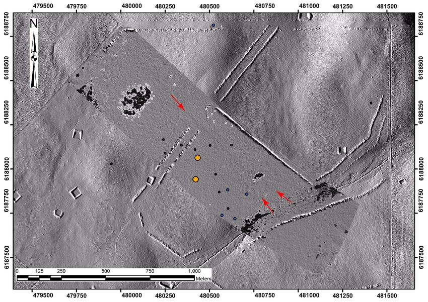
175 Figure S3. An example of a manual alignment of Lake Muir waveforms in GeoTool on the vertical component of station QIS.
Top to bottom: September, November and October events respectively. “X” picks represent old phase picks. “P” picks are
the new picks made after alignment, which is one pick made across all three events at the same time. The events were manually
aligned by dragging them so that key features (e.g. A, B, and C) are aligned between them. These waveforms have been
bandpass filtered 0.4-1.8 Hz (3rd order). While the P to X changes look small, the largest correction is 0.52 seconds. This
180 makes a significant difference when calculating a relative location.
Coulomb Stress modelling
When slip occurs on a fault (the ‘source’ fault) stress is imparted to the surrounding crust and faults (‘receiver’ faults). In
Coulomb stress modelling (e.g. Lin and Stein, 2004; Toda et al., 2005; Toda et al., 2011), fault displacements in the elastic
185 half-space are used to calculate a 3D strain field, which is multiplied by the elastic stiffness to derive stress changes. Stress
changes might be used to understand the distribution of aftershocks resulting from an event, or the static stress changes caused
by displacement on a ‘source’ fault can be resolved onto ‘receiver’ faults to investigate whether they are promoted towards
failure. The shear stress increase or decrease is dependent on the position, geometry, and slip of the source fault and on the
position and geometry of the receiver fault, including its rake. The normal stress change (clamping or unclamping) is
190 independent of the receiver fault rake (Toda et al., 2011).
Toda et al. (2011) use the Coulomb failure criterion, Δσf = Δτs + μ’ Δσn, in which failure is hypothesized to be promoted when
the Coulomb stress change is positive. Here, Δσf is the change in failure stress on the receiver fault caused by slip on the source
8fault(s), Δτs is the change in shear stress (reckoned positive when sheared in the direction of fault slip), Δσn is change in
normal stress (positive if the fault is unclamped), and μ’ is the effective coefficient of friction on the fault.
195
The source fault was parametrised as follows: length = 5 km, strike = 5°, dip = 50°, dip slip = 0.6 m, strike slip = 0.0 m, rake
= 90 °, top of rupture = 0 km, bottom of rupture = 0.9 km, co-efficient of friction (μ’) = 0.6 (Figures 8 and S4). The preferred
parametrisation for the strike-slip receiver fault (i.e. the November rupture plane) was determined through simple forward
modelling using a finite rectangular elastic dislocation model (Okada, 1985)
200 (https://earthquakes.aranzgeo.com/model/generic1). The Parameters that were found to best match the surface expression are
as follows: length = 4.1 km, strike = 233°, dip = 88°, dip slip = 0.0 m, strike slip = 0.4 m, rake = 0°, top of rupture = 1.0 km,
bottom of rupture = 2.5 km (Figure S5). This plane is shown in section on Figure S4b.
The Coulomb stress change consequent of the Lake Muir September MW 5.3 reverse fault rupture was resolved for optimally
oriented strike-slip events parallel to the plane of the November MW 5.2 strike-slip rupture (Figure S4). This calculation shows
205 that the plane of the November rupture was brought closer to failure over approximately half of its area, though only slightly
so in the hypocentral region.
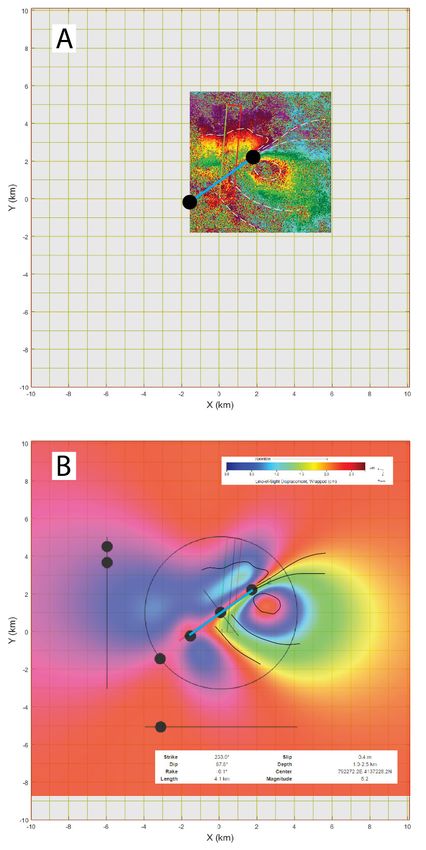
9Figure S4: Coulomb stress change resulting from the September event resolved for dextral strike-slip events onto the plane of the
210 November rupture. Stress increase values are shown in bars. The location and uncertainty ellipse of the hypocentre for the November
event is shown.
10Figure S5: Simple forward modelling of InSAR surface deformation envelope for the Lake Muir November mainshock. (a) InSaR
215 phase image (recoloured from Figure 6C to enhance fringes). Fringes used for matching are delineated with white dashes. Preferred
fault trace shown with a blue line ending in lack dots. (b) Forward model showing match to fringes (white dashed lines in part (a)
are reproduced as black lines).
11References
220 Agisoft LCC: . Agisoft PhotoScan Pro 1.4.3. Available online: http://www.agisoft.com (accessed November 2018).
Bratt, S. R., and Nagy, W.: The LocSAT Program, Science Applications International Corporation , San Diego, 1991.
Dentith, M. C., Dent, V. F., and Drummond, B. J.: Deep crustal structure in the southwestern Yilgarn Craton, Western
Australia, Tectonophysics, 325, 227-255, 2000.
Fisk, M. D.: Accurate Locations of Nuclear Explosions at the Lop Nor Test Site Using Alignment of Seismograms and
225 IKONOS Satellite Imagery, Bulletin of the Seismological Society of America, 92, 2911-2925, 10.1785/0120010268 %J
Bulletin of the Seismological Society of America, 2002.
Gindraux, S., Boesch, R., and Farinotti, D.: Accuracy Assessment of Digital Surface Models from Unmanned Aerial Vehicles’
Imagery on Glaciers, Remote Sensing, 9, 186, 2017.
Goldstein, P., Dodge, D., Firpo, M., Minner, L., Lee, W. H. K., Kanamori, H., Jennings, P. C., and Kisslinger, C.: SAC2000:
230 Signal processing and analysis tools for seismologists and engineers, The IASPEI International Handbook of Earthquake and
Engineering Seismology 81 1613-1620, 2003.
Kennett, B. L. N., Engdahl, E. R., and Buland, R.: Constraints on seismic velocities in the Earth from traveltimes, Geophysical
Journal International 122, 108-124, 1995.
Krischer, L.: hypoDDpy: hypoDDpy 1.0 Zenodo, 2015.
235 Lin, J., and Stein, R. S.: Stress triggering in thrust and subduction earthquakes and stress interaction between the southern San
Andreas and nearby thrust and strike-slip faults, Journal of Geophysical Research: Solid Earth, 109,
doi:10.1029/2003JB002607, 2004.
Lomax, A.: The NonLinLoc software guide, http://alomax.free.fr/nlloc ALomax Scientific, Mouans-Sartoux, France, 2008.
Okada, Y.: Surface deformation due to shear and tensile faults in a half-space, Bulletin of the Seismological Society of
240 America, 75, 1135-1154, 1985.
Ouédraogo, M. M., Degré, A., Debouche, C., and Lisein, J.: The evaluation of unmanned aerial system-based photogrammetry
and terrestrial laser scanning to generate DEMs of agricultural watersheds, Geomorphology, 214, 339–355, 2014.
Pujol, J.: Joint Event Location — The JHD Technique and Applications to Data from Local Seismic Networks, in: Advances
in Seismic Event Location, edited by: Thurber, C. H., and Rabinowitz, N., Springer Netherlands, Dordrecht, 163-204, 2000.
245 Rajabi, M., Tingay, M., Heidbach, O., Hillis, R., and Reynolds, S.: The present-day stress field of Australia, Earth-Science
Reviews, 168, 165-189, 10.1016/j.earscirev.2017.04.003, 2017.
Salmon, M., Kennett, B. L. N., and Saygin, E.: Australian Seismological Reference Model (AuSREM): crustal component,
Geophysical Journal International, 192, 190-206, 10.1093/gji/ggs004 %J Geophysical Journal International, 2012.
Sambridge, M. S., and Kennett, B. L. N.: Seismic event location: nonlinear inversion using a neighbourhood algorithm, Pure
250 and Applied Geophysics 158, 241-257, 2001.
Seitz, S. M., Curless, B., Diebel, J., Scharstein, D., and Szeliski, R.: A comparison and evaluation of multi-view stereo
reconstruction algorithms, In Proceedings of the 2006 IEEE Computer Society Conference on Computer Vision and Pattern
Recognition (CVPR’06), New York, NY, USA, 17–22 June 2006, 1, 2006.
Serifoglu Yilmaz, C., Yilmaz, V., and Güngör, O.: Investigating the performances of commercial and non-commercial
255 software for ground filtering of UAV-based point clouds, International Journal of Remote Sensing, 39, 5016-5042,
10.1080/01431161.2017.1420942, 2018.
Toda, S., Stein, R. S., Richards-Dinger, K., and Bozkurt, S. B.: Forecasting the evolution of seismicity in southern California:
Animations built on earthquake stress transfer, 110, 10.1029/2004jb003415, 2005.
Toda, S., Stein, R. S., Sevilgen, V., and Lin, J.: Coulomb 3.3 Graphic-Rich Deformation and Stress-Change Software for
260 Earthquake, Tectonic, and Volcano Research and Teaching — User Guide, USGS Open File Report, 2011-1060, 63p, 2011.
Tonkin, T. N., and Midgley, N. G.: Ground-Control Networks for Image Based Surface Reconstruction: An Investigation of
Optimum Survey Designs Using UAV Derived Imagery and Structure-from-Motion Photogrammetry, Remote Sensing, 8, 1–
8, 2016.
12Waldhauser, F., and Ellsworth, W. L.: A Double-Difference Earthquake Location Algorithm: Method and Application to the
265 Northern Hayward Fault, California, Bulletin of the Seismological Society of America, 90, 1353-1368, 10.1785/0120000006
%J Bulletin of the Seismological Society of America, 2000.
Waldhauser, F.: HypoDD: A Computer Program to Compute Double-difference Hypocenter Locations, USGS Open File
Report 25, 1–113, 2001.
Williams, R.: DEMs of difference, Geomorphological Techniques, 2, 2012.
270 Zhang, W., Qi, J., Wan, P., Wang, H., Xie, D., Wang, X., and Yan, G.: An Easy-to-Use Airborne LiDAR Data Filtering Method
Based on Cloth Simulation, Remote Sensing, 8, 501, 2016.
13You can also read