A New Crescent Moon Visibility Criteria using Circular Regression Model: A Case - UKM

Sains Malaysiana 49(4)(2020): 859-870
http://dx.doi.org/10.17576/jsm-2020-4904-15

 A New Crescent Moon Visibility Criteria using Circular Regression Model: A Case
 Study of Teluk Kemang, Malaysia
 (Kriteria Baru Kebolehnampakan Bulan Sabit menggunakan Model Regresi Berkeliling: Suatu Kajian Kes Teluk
 Kemang, Malaysia)

 N azhatul s hima A hmad*, M ohd S aiful A nwar M ohd N awawi, M ohd Z ambri Zainuddin, Z uhaili M ohd
 N asir, R ossita M ohamad Y unus & I brahim M ohamed

 ABSTRAct
Many astronomers have studied lunar crescent visibility throughout history. Its importance is unquestionable, especially
in determining the local Islamic calendar and the dates of important Islamic events. Different criteria have been used
to predict the possible visibility of the crescent moon during the sighting process. However, so far, the visibility models
used are based on linear statistical theory, whereas the useful variables in this study are in the circular unit. Hence, in
this paper, we propose new visibility tests using the circular regression model, which will split the data into three
visibility categories; visible to the unaided eye, may need optical aid and not visible. We formulate the procedure to
separate the categories using the residuals of the fitted circular regression model. We apply the model on 254 observations
collected at Baitul Hilal Teluk Kemang Malaysia, starting from March 2000 to date. We show that the visibility test
developed based on elongation of the moon (dependent variable) and altitude of the moon (independent variable) gives
the smallest misclassification rate. From the statistical analysis, we propose the elongation of the moon 7.28°, altitude
of the moon of 3.33° and arc of vision of 3.74 at sunset as the new crescent visibility criteria. The new criteria have a
significant impact on improving the chance of observing the crescent moon and in producing a more accurate Islamic
calendar in Malaysia.

Keywords: Circular regression; crescent moon; lunar month; q-test; visibility criteria

 ABSTRAk
Ramai ahli astronomi telah mengkaji kebolehnampakan bulan sabit sepanjang sejarah. Kepentingannya tidak dapat
dipertikaikan, terutama dalam menentukan kalendar Islam tempatan dan tarikh peristiwa penting Islam. Kriteria yang
berbeza telah digunakan untuk meramalkan kemungkinan kebolehnampakan bulan sabit semasa proses pencerapan.
Walau bagaimanapun, setakat ini, model kebolehnampakan yang digunakan adalah berdasarkan teori statistik linear,
sedangkan pemboleh ubah penting dalam kajian ini adalah dalam sukatan membulat. Oleh itu, dalam kertas ini, kami
mencadangkan ujian kebolehnampakan baru menggunakan model regresi berkeliling, yang akan membahagikan data
menjadi tiga kategori kebolehnampakan; dapat dilihat dengan mata kasar, mungkin memerlukan bantuan optik dan
tidak kelihatan. Kami memformulasi prosedur tersebut untuk memisahkan kategori menggunakan sisa model regresi
berkeliling yang sesuai. Kami mengaplikasikan model tersebut dalam 254 pemerhatian yang dikumpulkan di Baitul Hilal
Teluk Kemang Malaysia, bermula dari Mac 2000 sehingga kini. Kami menunjukkan bahawa ujian kebolehnampakan
dibangunkan berdasarkan pemanjangan bulan (pemboleh ubah bersandar) dan ketinggian bulan (pemboleh ubah
bebas) memberikan kadar salah pengkelasan terkecil. Daripada analisis statistik, kami mencadangkan pemanjangan
bulan pada 7.28°, ketinggian bulan 3.33° dan aras penglihatan 3.74° ketika matahari terbenam sebagai kriteria
baharu kebolehnampakan bulan sabit. Kriteria baharu ini memberi kesan yang besar dalam meningkatkan peluang
melihat bulan sabit dan menghasilkan kalendar Islam yang lebih tepat di Malaysia studied.

Kata kunci: Bulan lunar; bulan sabit; kriteria kebolehnampakan; regresi berkeliling; ujian q

 i ntroduction moon is of utmost importance since the time of Babylon
 Era (Ilyas 1994). The criteria are mainly derived based on
Main religions in the world, including Jews, Hindu, and
 the crescent moon data collected at end of the month. The
Islam, have their calendars based on lunar month. They
 variables measured include elongation (Elon), altitude of
are mainly used to determine dates of important events or
 the moon (Alt(M)), altitude of the sun (Alt(S)), arc of vision
festivals in each religion. As a result, the determination of
 (ARCV), width of the crescent moon (W), lag time between
criteria to indicate the expected visibility of the crescent
 sunset and moonset (lag time), and age of the crescent

860

moon from conjunction (age). The choice of the parameters is supposed to be 5° rather than 7°. However, Schaefer
for the criteria mainly correspond to the minimum contrast (1991) explained that atmospheric seeing is not the
between the brightness of the moon and the sky. That is, main factor in the deficiency of the arc. He developed a
we look at certain values such that the moon is bright model and suggested 7° as the new Danjon limit for the
enough, or the sky is dark enough for the crescent moon crescent to be visible. Ilyas (1983) stated that the Danjon
to be seen. For example, the Babylonians used age and lag limit is intended to be a general guide. However, for the
time as a measure of brightness of the moon and the sky, formation of calendar regulation, elongation of 10.5° is
respectively (Bruin 1977). Here the lag time is at least 48 the best. Fatoohi et al. (1998) and Odeh (2004) studied
min after sunset, and this value has changed since. the observational reports and respectively concluded
 In the past, different studies report the criteria based that 7.4° and 6.4° as the estimated Danjon limits. Sultan
on a different set of variables measured in crescent moon (2007) and Hasanzadeh (2012) developed a photometric
sighting activities. Among the early Arabic astronomers, model of crescent visibility and re-evaluated the Danjon
Al-Tabari utilized the depression angle of the sun in the limit to be 5°.
visibility of the crescent moon. The crescent would be Different mathematical approaches have been used to
considered visible at the time of moonset if the altitude of arrive at the values the criteria. McNally (1983) studied
the sun was 9.5° below the horizon (Guessoum & Meziane mathematically the effect of atmosphere on the shape of
2001; Hogendijk 1988). In the more recent centuries, most crescent moon and formulated the width as a measure of
models were built based on the observations made by Julius shortening the crescent moon in terms of θ and φ, where θ
Schmidt in Athens, Greece, from 1859-1880 (Schaefer =180-χ, χbeing the elongation of the earth from the sun as
1988). Based on 76 sets of observations of the crescent
moon, Fotheringham (1910) established necessary viewed from the moon centre and φ is the position of outer
specific criteria, which include the relative altitude of the terminator near the cusp. He suggested the atmospheric
moon with respect to the sun’s altitude (known as an arc factor should be considered in order to maximize the
of vision, ARCV). By placing a line of separation between length of the outer terminator. The poor seeing condition
the negative and positive crescent moons, Fotheringham will cause a shortened terminator of the crescent moon.
(1910) gave a minimum limit of an ARCV of 12° and However, Schaefer (1991) later argued that atmospheric
a relative azimuth of 0°. Maunder (1911) formulated a factor is not important by considering the Hapke’s lunar
smaller minimum limit than Fotheringham (1910), which surface brightness measure.
is 11° ARCV at 0° relative azimuths, for when the crescent Ilyas (1994) reviewed the development of criteria,
moons can be seen, as he suggested there was a technical especially in producing universal international Islamic
issue with the negative data reported by Fotheringham. calendar amid the challenge for quality crescent moon
Ilyas (1988) examined the ACRV and its relative azimuth data. A unified approach of five practical considerations
criteria and found the criteria proposed by Fotheringham is proposed to come up with a universal international
(1910) and Maunder (1911) were limited to a difference Islamic calendar in the future. Yallop (1997) introduced
in azimuth of 20°. At a larger scale, these criteria cannot be the q-test as a test of the visibility of the crescent by
applied. Consequently, to match his criteria of elongation considering the residuals of the fitted polynomial
of 10.4°, Ilyas (1988) concluded that the minimum limit regression model of ARCV on the width of crescent moon.
of ARCV was supposedly 10.5° with a relative azimuth Several different categories of visibility are proposed.
of 0°. Recently, Raharto et al. (2019) presented the all- Hoffman (2003) provided a collection of crescent moon
possible moon astronomical position at sun-set time in a data set observed in good weather conditions. He used
diagram of Alt(M) vs Elon and the azimuth difference of to update the criteria of the q-test and further claimed
the moon and the sun. Then, by analysing the importance that the data could be used to validate any visibility tests.
of different variables considered in the study, they came Similarly, Odeh (2004) combined data set from different
up with a set of new criteria based on the arc of light with studies and used them to come up with the new values of
values 6° or 6.4° depending on the visibility on equatorial the existing criteria. Hasanzadeh (2012) used the weighted
and subtropical observation. polynomial function of the arclength of crescent moon
 In recent years, discussion on the criteria focussed against elongation and obtained a new value of the
on the Danjon limit (Danjon 1936). In the year 1931, the Danjon limit by extrapolating the curves to the case of
French astronomer André Danjon measured 75 moon zero arc length. Recently, Alrefay et al. (2018) analysed
samples observed using a theoretical approach. He the relationship between different pair of variables. In
estimated the length of the crescent moon by measuring particular, they proposed the hypothetical curve which can
the parts of the moon illuminated by sunlight. Crescent best separated the observations with positive/negative
is expected to be visible if the elongation is more than crescent moon visibility in terms of W and ARCV.
7°, hereafter known as the Danjon limit (Fatoohi et al. So far, the development of the criteria uses only
1998). Further improvement of the criteria was later linear statistical theory. However, most of the variables in
published. McNally (1983) suggested that atmospheric crescent moon data are measured in degree/radians. Hence,
seeing causes the crescent to be obscured when it is smaller in this paper, we consider the circular statistical theory
than the seeing disk. He concluded that the Danjon limit to come up with new criteria for the visibility of local

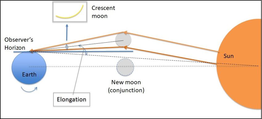
861

crescent moon data. The proposed criteria follow closely Zulkaedah of Hijr) each year to determine the start of the
the methods adopted by Yallop (1997) for the q-test. This fasting month, Eid al-Fitr and Eid al-Adha, until 1999.
paper is organized as follows: In the next section, we The observations were conducted using theodolites
present the background of the data collected at the main operated by the surveyors and the committee of crescent
observing station in Malaysia. Then, the circular statistical moon observation to validate the visibility if it is
theory used in this study is covered in subsequent section sighted. Starting in March 2000, the observation has
while the development of the new tests is in section that been carried out consistently on the 29th and 30th of
follows. In the following section, we presents the findings each lunar months until now. We used various equipment
of the study. Discussion on the results and conclusion are and methods in the observations, such as theodolites,
included in the last section. portable telescopes of 12-inch reflector and 76 mm
 refractor, and the naked eye. The images of the crescent
 OBSERVATIONS AND DATA COLLECTION moon were then recorded using a DLSR camera.
We carried out the crescent moon sighting activities We have collected 254 data since 2000 (1420H)
at Baitul Hilal Teluk Kemang (Latitude: 2° 27’ 44” N, which consists of 81 positive data, and the rest of the
Longitude: 101° 51’ 21”E, height: 14 m above sea level). data are not visible due to bad weather and severe
Historically, this site was the first location in Malaysia sky conditions, and due to the very low values of the
used for sighting the crescent moon in the 1970s. criteria to be observed. Table 1 and Figure 1(a) and 1(b)
During the years, the observations were conducted only respectively show the definition and diagram of the
for three lunar months (29th of Ramadhan, Syawal, and geometric variables used for the sun and moon.

 table 1. The definition of geometric variables used for the sun and moon

 Variable Definition
 W Width of the crescent moon as view from the earth, measured in
 arcminutes

 Alt(S) Altitude of the sun

 Alt(M) Altitude of the moon

 ARCV Arc of vision, i.e. the geocentric difference in the altitude between the
 centre of the sun and the centre of the moon for a given latitude and
 longitude with taking into account the effects of refraction
 Elon Elongation, which refers to the angle between the centre of the sun
 and the centre of the moon, as viewed from earth

 Status Y = visible, N = not visible

 figure 1 (a). Schematic diagram of geometric variables of the Sun and moon at sunset: ARCV, relative
 altitude between the center of the moon and the sun; ALT, altitude of the center of the crescent moon above the
 horizon; DAZ, azimuth difference between the sun and moon; ARCL is equivalent to elongation; and Width,
 the crescents width

862

 figure 1 (b). Global view of the geometric variables of the sun and moon after a few hours of conjunction;
 Elongation is an angle between the center of the sun and the moon as seen from the Earth and the reflected of
 light from the moon after several hours of conjunction called the crescent

 METHODS
We note that the five variables considered in Table 1 are  tan 1 ( S C ), if S  0, C  0,
  
circular; that they are measured in radian or degree. One  , if S  0, C  0, (1)
of the important properties of circular variables is the  2
    tan -1 ( S C )   , if C  0,
bounded property of the variables such that the observed  -1
values taken are within the range (0, 2π). Recent papers tan ( S C )  2 , if S  0, C  0,
in circular regression models and their diagnostic tools  undefined, if S  0, C  0.
 
include Alkasadi et al. (2018) and Kim and Rifat
(2019). Here, we intend to use the relevant theory in One of the mean direction characteristics is that
 ∑ sin (θ i − θ ) = 0 , which is analogous to the linear case.
 n
circular statistics in order to come with a better visibility
 i =1
test for crescent moon detection. Detail is available in
Jammalamadaka and SenGupta (2001).
 Concentration parameter
 MEASURES FOR CIRCULAR VARIABLES
 The concentration parameter, denoted by κ , is a standard
To describe any circular data set, we need some measures measure of dispersion for c distribution. Best and Fisher
of location and dispersion. Let θ1 ,..., θ n be observations (1981) gave the maximum likelihood estimates of the
in a random circular sample of size n from a circular concentration parameter κ as follows:
population.
  2R 2R R3R536R55 , R 5 , if if  0.R53 0.53
 R
Mean direction  
 
 6
 ˆ    4  1 . 39 R  0 . 43 0
 ˆ   0.4  1.39 R  1  R 
 0 . . 43 , , if .530.R85 0(2)
 if0.53 0R .85
  3 1 R 
To summarize the circular data, we use the mean  R 3 2
   1
  R4 R 4R3R  3,R ,
 2 1
   if ifR  0.R85 0.85
direction as a measure of tendency. For a given circular
random sample, we consider each observation to be a
 R
unit vector whose direction is specified by the circular where R is mean resultant length and is given by R = .
angle and find their resultant vector. The mean direction n
 The larger the value of concentration parameter, the more
is defined by the angle made by the resultant vector with a concentrated the data towards the mean direction.
horizontal line. Specifically, we have the resultant length
 R given by, Median, quantile and percentile
 2 2
 R= C +S , Mardia and Jupp (1972) defined the median as any point
 n n φ , where half of the data lie in the arc [φ , φ + π ) and
where C = ∑ cos θ i and S = ∑ sin θ i . The mean direction, the other points are nearer to φ than to φ + π . Basically,
 i =1 i =1
 C for any circular sample, Fisher (1993) defined the
θ , may be obtained by solving the equations, cos θ =
 S R median direction as the observation which minimizes
and sin θ = , where the summation of circular distances to all observations
 R n
 θ1 ,..., θ n , that is, d (φ ) = π − ∑ π − θ i − φ . Fisher’s
 i =1

863

definition is used to obtain the circular median in the We may then predict v such that
Oriana statistical software package. On the other hand,
the first and third quantile directions Q1 and Q3 are any tan tan −12 ( ) 2
 −1
 −1 ( ) 2
 ( )
 ( )
 10( )
 01 ( )
 ( ) 0> > 0
 tan ( )
 >> 0
 −1 2 2 ( )
 tan
 tan −1
 ( ) 1 ( ) 1 ( )
 1>
solution of 1 1( ) 1 ( )
 ( )
 1
 1

 2 ( )
 0(7)
 
 ( )
 ( )
 22( ) ( )
 −1 −12 −12 ( ) ( )
 22( )
 2 ( )
 =
 10( )
 ( )== ̂̂ ̂̂=
 == ( )1≤
 ( )
 ( ) = ̂arctan
 = arctan
 arctan
 arctan = == +++tan
 ++−1tan
 tan 
 1 0≤
 ( ) ≤ ≤≤0 0
 ( )
 2−1
 ( ) = arctan tan 1 ( )
 2
 ( ) = 1 ( )
 ( )
 =
 1 ( )
 tan 1 ( )
 1 ( ) 
 ( ) ( )
 1( ) 1 ( )
    Q3 1 1( )
 1 ( ) 1 1
 ( ) =
 2=( ) =( )
 0 =0
  f ( )d  0.25 and  f ( )d  0.25
 
 (3) 
 
 1 1 ( )
 =
 1 ( )
 
 1 1 ( ) =
 ( )
 2 =
 2 ( )
 2 2 0 ( )
 =( ) = 0= 0
  Q1
 The difficulty of non-parametrically estimating
respectively. Q1 can be considered as the median of the g1(u) and g2(u) leads us to approximate them by using
first (3)
 half of the ordered data and Q3 as the median of the suitable functions, taking into account they are both
second. The percentiles can then be obtained by further periodic with period 2π. The approximations used are
splitting the ordered sample. the trigonometric polynomials of suitable degree m of the
 form
 CIRCULAR CORRELATION

Special measure of correlation has been developed for 1 ( ) ≈ ∑ 
 =0( cos + sin )
any two circular variables. Given ( 1 , 1 ), … , ( , ) is
a random sample of observations measured as angles. =0( cos
 2 ( ) ≈ ∑ + sin ) (8)
As for measuring the correlation between two circular
variables, we use the sample circular correlation given by We therefore have the following models:

 cos = ∑ 
 =0( cos + sin ) + 1
 � � sin t �
 � sin t
 � t
 (4)(4) sin = ∑ 
 =0( cos + sin ) + 1 (9)
 � � � � � �
 � sin � sin t t
 where ε  ( 1 ,  2 ) is the vector of random errors following
where and are sample mean directions. As in the linear the normal distribution with mean vector 0 and
case, takes values in the range and the closer to 1 or -1 unknown dispersion matrix Σ. The parameters Ak, Bk, Ck,
indicates the stronger relationship between the variables. and Dk, where k = 0, 1, …, m, the standard errors as well
The relationship for circular variables can also be as the dispersion matrix Σ can then be estimated using
described using spoke plot (Zubairi et al. 2008). the generalized least squares estimation method. As for
 the errors, we use the definition of circular distance as
 given Jammalamadaka and SenGupta (2001) such that,
 CIRCULAR REGRESSION MODEL

Due the bounded property of circular variables, various = π − | − | − ̂ || (10)
circular regression models have been proposed to model
the relationship between 2 circular variables, see
 = πfor | − ̂ |is
 − | −where | the estimated value of v.
example in Hussin et al. (2004). Here, due to its simple
property and possibility to be extended to a general
 THE CRESCENT MOON VISIBILITY TESTS
case, we consider the regression model proposed by
Jammalamadaka and Sarma (1993), (JS hereafter) for In this section, we revisit the q-test proposed by Yallop
two circular random variables U and V in terms of the (1997) and propose new tests based on circular regression
conditional expectation of e given u given by,
 (iv) model.

 THE Q-TEST
 ��� �� �
 � � � � �� � � ��� � (5)
 In developing new crescent moon visibility tests using
 circular regression model, we follow closely the q-test
where e iv = cos v + i sin v, ( ) represents the conditional of Yallop (1997). The test is based on the topocentric
mean direction of v given u and p(u) the conditional crescent width, W, and geocentric ARCV. Yallop’s
concentration parameter for some periodic function g1(u) algorithm computed crescent visibility based on the
and g2(u). Equivalently, we may write residuals resulting from the fitted polynomial regression
 ̂ = =11.8371
 11.8371− -6.3226 
 6.3226W+ +0.7319
 0.7319W
 2 −2 -0.1018 
 0.1018W 3 3

 on 295 observations compiled by Schaefer (1996). The
 (cos | ) = 1 ( ) (6) residuals are then divided by 10 giving the q-statistic,
 (sin | ) = 2 ( ) ̂ ]

 =
 [ − 
 . (11)
 10

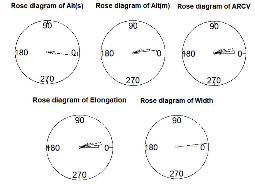
864

He further defined five different categories depending on and non-visible categories for q < −0.293 as described in
the visibility of crescent moon using various instruments Table 2.

 table 2. The q-test types by Yallop (1997)

 Types q-test value Justification
 A q > +0.216 Easily visible to the unaided eye (≥ 12ARCV)

 B –0.014 < q < +0.216 Visible under certain atmospheric conditions

 C –0.160 < q < –0.014 May need optical aid to find the thin crescent
 moon before it can be seen with the unaided eye

 D –0.232 < q < –0.160 Can only be seen with binoculars or a telescope

 E –0.293 < q < –0.232 Below the normal limit for detection with a
 telescope

 F q < –0.293 Not visible below the Danjon limit

 Hoffman (2003) investigated the validity of As in the q-test, we use the resulting residuals from the
the Yallop (1997) criteria using the results of 539 JS circular regression model on two circular variables to
observations of the moon made over several years by categorize the visibility of the crescent moon. We then
many experienced observers in good weather conditions. attempt to classify the residuals into different groups and
The data were selected from 1047 reports. He proposed relate the groups according to the visibility of the crescent
a three-category of visibility type namely; the crescent moon. We achieve that by taking the following steps:
moon is visible if q is higher than 0.43 and not visible First, find the 99%, 95%, and 90% confidence
if q is less than −0.06. These suggest that different data intervals of the residuals, namely [L99, U99], [L95, U95]
set may give different ranges of the categories. and [L90, U90], respectively. Next, form 7 categories,
 We also applied the same q-test on our 254 data, namely (−∞, L99], (L99, L95], (L95, L90], (L90, U90],
and we found that the lowest value of the q-test with (U90, U95], (U95, U99], (U99, ∞). After that, tabulate the
a positive crescent sighting is −0.347. This value is frequency of crescent moon visibility/non-visibility for
significantly lower than the minimum limit of the q-test each category. Lastly, reduce the number of categories
by Yallop (1997). Though the q-test value is lower, the based on the tabulated frequencies.
elongation of the crescent moon is 11.33°, which is In cases considered, we reduced the categories into
higher than the Danjon limit. The inconsistent values of three groups associated with ‘Visible to the unaided
the test make this q-test very subjective, and the value eye’, ‘May need optical aid’, and ‘Not visible’. These
cannot be used as a standard limit for crescent moon categories will then be finalized, and the performance of
visibility. the test is investigated.

 THE NEW CRESCENT MOON VISIBILITY TEST RESULTS AND ANALYSIS
The main interest of this work is to find alternative CIRCULAR DESCRIPTIVE ANALYSIS
crescent visibility tests besides the q-test.The new test is
developed by generalizing the derivation of the q-test by The distribution of the values of the circular variables
Yallop (1997) based on the circular regression model. can be described by a rose diagram, as depicted in Figure
The new crescent moon visibility test utilizes two 2. The data are mainly concentrated and close to zero.
circular variables, say U and V only. We fit the variable These show the condition of an early phase of the moon
U on V using the JS circular regression model, as after the sunset. Table 3 provides the mean, minimum/
described in Circular Regression Model section, giving maximum, and the 95% confidence interval (CI) for the
 ̂, the fitted values of ̂,. Hence, we define the UV-statistic circular variables. As expected, the width of the crescent
as moon during sighting is generally minimal, and the
 altitude of the moon is mostly above the horizon though
 = π − | − | − ̂||. (12) ARCV is more substantial than the altitude of the moon
 because ARCV considers the position of the sun below the
 horizon.

865

 table 3. Summary statistics for linear/circular variables

 Mean direction (min, max) 95% CI
Variable
 (degree) (degree) (degree)

Width 0.006 (0,0. 0.032) (0.005, 0.007)

Alt(S) -1.652 (-19.934, 4.019) (-2.094, -1.274)

Alt(M) 7.498 (-5.460, 27.835) (6.791, 8.204)

ARCV 9.159 (-5.165, 26.405) (8.440, 9.957)

Elon 10.779 (0.563, 28.244) (10.099, 11.527)

 table 4. Circular correlation between circular variables

 Variable W Alt(S) Alt(M) ARCV Elon

W

Alt(S) -0.233

Alt(M) 0.827 0.212

ARCV 0.924 -0.334 0.850

Elon 0.962 -0.287 0.841 0.966

 figure 2. Rose diagrams of the circular variables

866

 We also calculated the correlation values between other variables (Hoffman 2003). Hence, in this paper,
the variables, which are tabulated in Table 4. We found we use the combination of Elon-Alt(M), and Elon-ARCV.
that the correlation values of Alt(M)-W, ARCV-W, Elon- Figures 3 and 4 give the plots of Elon against Alt(M)
Width, ARCV-Alt(M), Elon-Alt(M), and Elon-ARCV are and ARCV, respectively. The altitude of the moon for
high. Nevertheless, not all the highly correlated variables Y visibility is recorded at the time of the moon being
are suitable to be used as the parameters for crescent sighted, which occurs a few minutes after the sunset. In
visibility. Based on the description of variables as given this case, the Sun’s altitude is at several degrees below
in Figure 1, ARCV-Alt(M) and Elon-W are expected to the horizon. Whereas for N visibility, the altitude of the
be highly correlated as they are collinear to each other. moon is calculated at sunset. Therefore, the distribution
Thus, they are not a good combination of variables for of data for Y is expected to be more scattered than N cases.
the visibility criteria. As for width, the variation of the From both plots, we observed that the larger the values
values is too small and might affect the relationship with of Elon, ARCV, and Alt(M), the higher the possibility of
 sighting the crescent moons.

 figure 3. Elon versus the Alt(M) variables figure 4. Elon versus the ARCV

 THE NEW VISIBILITY TEST

For these new visibility test, we use the combination of Using the approach adopted by Yallop (1997), we
variables as discussed in Circular Descriptive Analysis define the EA-test, which takes values of residuals of the
section. They are Elon-Alt(M), and Elon-ARCV. We fitted JS circular regression model. We then attempt to
compare the performance of the two new visibility tests categorize EA using the procedure described in EA-test
by the misclassification percentage of the data. section as tabulated in Table 5. The second column gives
 the intervals of the categories based on the EA-test; for
EA-test example, Category A consists of observations with EA
 greater than 0.0086. The third and fourth columns give
The new crescent moon visibility test, called EA-test, the frequency of crescent moon non-visibility (N) and
utilizes two circular variables Elon, E, and Alt(M), A. visibility (Y). For Category A, the number of Y is greater
The best fitted JS circular regression model with m=1 than N, while for Category C, more N compared to Y.
is given by Hence, we label Category A as ‘Visible to the unaided
 eye’ while Category C as ‘Not visible’. As for Group
 B, the number of N and Y are fewer with smaller Y
 cos ̂ = 0.1832 + 0.8104 cos − 0.0372 sin (13) compared to N. This might be due to many reasons
 sin ̂ = 1.0108 − 0.9178 cos + 0.6172 sin . including the condition of the sky, and hence labelled
 as ‘May need optical aid’. The percentage of correct
 classification for the EA-test is 70.10%.

 table 5. Distribution of moon visibility based on three categories

 Category EA-test value N Y Total % Interpretation
 A [0.0086, ∞) 21 52 73 (29) Visible to the unaided eye
 B [-0.00516, 0.0086) 26 9 35 (14) May need optical aid
 C (-∞, -0.0052) 126 20 146 (57) Not visible

867

 Figure 5 gives the plot of EA versus Alt(M). It shows cos ̂ = −0.0480 + 1.0452 cos − 0.0021 sin (14)
that the residuals separate the Y/N values quite well.
Observations with low residuals and small Alt(M) are sin ̂ = 1.5536 − 1.4884 cos + 0.5877 sin 
largely categorized as non-visible, which is below
-0.00156. For EA above 0.0086, the moon can be observed Using the same approach as for the EA-test, the final
by unaided eyes. Otherwise, an optical aid may be need- categories are given in Table 6. The EV-test does not
ed in the sightings. give a good result, with the percentage of correct clas-
 sification is only 43.7%. This low performance is sup-
EV-test ported by the plot of EV versus ARCV, as given in Figure
 6. The distribution of the residual values of Y and N data
We repeat the process using the Elon and ARCV, V, are more scattered than that of the EA-test; thus, it fails
denoted as EV-test. The best fitted JS regression model to separate the Y and N data very well.
with m=1 is given by

 table 6. Distribution of moon visibility based on three categories

 Category EV-test value N Y Total % Interpretation
 A [0.0039, ∞) 59 21 80 (31) Visible to the unaided eye

 B [-0.0022, 0.0039) 24 16 40 (16) May need optical aid
 C (-∞, -0.0022) 90 44 135 (53) Not visible

 figure 5. EA-test versus the Alt(M) figure 6. EV-test versus the ARCV

 d iscussion and, hence, the choice of 15% percentile seems to be
 adequate for this data. The five observations are listed in
The results in Results and Analysis section indicate
 Table 7. Most of them have rather low values of Alt(M)
that EA-test provides the best indicator of visibility of
 and ARCV, which makes it rather difficult to sight the
the crescent moon because of the higher percentage of
 crescent moon after the sunset. Hence, the value of the
correct detection. Hence, we attempt to come up with
 criteria for Elon is estimated at 7.28°.
the new visibility criteria based on the EA-test. The lower
 As for Alt(M) and ARCV, we consider the plot of
limit of the variables is then used as the criteria. In this
 Elon-Alt(M) and Elon-ARCV, as shown in Figures 7 and
work, the criteria will be based on Category B of Table 5
 8, respectively. We then estimate the corresponding values
as nowadays, telescopes or other optical aid systems are
 of Alt(M) and ARCV given that Elon = 7.28°. Hence,
used in the observations. As Elon is taken as the dependent
 the values are Alt(M) and ARCV are 3.03° and 3.74°,
variable in the EA-test, we first estimate the criteria
 respectively. Consequently, by definition, the estimated
value of Elon by its percentile values. The 5th, 10th, and
 Alt(S) is taken as the difference between ARCV and
15th percentile mean 5%, 10%, and 15% of the ordered
 Alt(M), that is -0.71°. As for W, the observed values are
observations will be smaller than the percentile values,
 consistently small and we use the 15th percentile as its
respectively. That corresponds to 1, 3, and 5 observations
 estimate, which is 0.1°. We note that the sun’s altitude

868

of 0.71° below the horizon has considered the effect of sunset is considered negligible to elongation as the average
refraction near the horizon and semi-diameter of the sun. rotation rate of the moon surrounding the earth takes
During sunset, the centre of the sun is estimated at 0.35° about 0.008°/min. Hence, the adjusted values of criteria
below the horizon, and hence the estimated time taken for for Elon and Alt(M) are 7.34° and 3.33°, respectively, and
the sun to the altitude -0.71° is 1.4 min after it sets. the corresponding values for ARCV = 3.74° and Alt(S) =
 In determining the final value for the crescent visibility -0.35. The final new values of the crescent moon visibility
criteria, we use the elongation and altitude of the crescent criteria are as listed in Table 8.
moon at sunset. We note that the duration of 1.4 min after

 table 7. Observations with Elon less than the 15th percentile value

 Date of Date of moon Elon Alt(M) ARCV (°) Alt(S) Width Visibility
 moon sighting (Hijr) (°) (°) (°) (°) (Y/N)
 sighting
 27.07.2014 29 Ramadan 7.042 2.577 2.912 -0.335 0.11 N
 1435
 10.11.2007 29 Syawal 6.898 1.963 2.314 -0.351 0.11 N
 1428
 16.09.2012 29 Syawal 6.286 0.945 1.361 -0.416 0.1 N
 1433
 25.04.2009 29 6.276 1.286 1.495 -0.209 0.1 N
 Rabiulakhir
 1430
 27.06.2014 29 Syaaban 4.888 -0.319 0.114 -0.433 0.05 N
 1435

 table 8. The values of new criteria of variables for Category B of the EA-test at sunset

 Variables Value of criteria (°)
 Elon 7.28

 Alt(M) 3.33
 ARCV 3.74

 Alt(S) -0.35
 Width 0.10

 figure 7. Elon vs Alt(M) for observations Category B of the figure 8. Elon vs ARCV for observations in Category B of the
 EA-test EA-test

869

 c onclusion parameters. Communication in Statistics - Simulations and
 Computations 10(5): 394-502.
We consider 254 observations collected consistently Bruin, F. 1977. The first visibility of the lunar crescent. Vistas
every month at Baitul Hilal Teluk Kemang Malaysia in Astronomy 21(4): 331-358.
for the past 19 years. We derive two new visibility tests Danjon, A. 1936. Ann. L’Obs. Strasbourg 3: 139-181.
based on elongation, the altitude of moon and ARCV Fatoohi, L.J., Stephenson, F.R. & Al-Dargazelli, S.S. 1998. The
of the crescent moon. We divide the test values into Danjon limit of first visibility of the lunar crescent. The
three categories, namely, crescent moon visible by the Observatory: A Review of Astronomy 118: 65-72.
naked eye, visible with optical aid, and not visible. Fisher, N.I. 1993. Statistical Analysis of Circular Data. London:
The new criteria are defined based on the observation Cambridge University Press.
 Fotheringham, J.K. 1910. On the smallest visible phase of the
of the second category, visible with optical aid. We use
 moon. Monthly Notices of the Royal Astronomical Society
the 15th percentile value to be the value of criteria for
 70: 527-531.
elongation and width. We then estimate the criteria values Guessoum, N. & Meziane, K. 2001. Visibility of the thin lunar
of the altitude of the moon and ARCV by utilizing the crescent: The sociology of an astronomical problem (A
relationship between Elon-Alt(M) and Elon-ARCV. The case study). Journal of Astronomical History & Heritage
criteria are further adjusted so that the elongation and 4: 1-14
altitude of the crescent moon are measured at sunset. We Hasanzadeh, A. 2012. Study of Danjon limit in moon crescent
use the 15th percentile of the elongation and width and sighting. Astrophysics and Space Science 339: 211-221.
propose the elongation of 7.28 and the width of 7.1 as Hoffman, R.R. 2003. Observing the new moon. Mon. Not. R.
the new criteria for new crescent moon visibility. Then, Astron. Soc. 340: 1039-1051.
we obtain another two criteria values, the altitude of the Hogendijk, J.P. 1988. New light on the lunar visibility table
 of Yaʿqub ibn Tariq. Journal of Near Eastern Studies 47:
moon of 3.38, and ARCV of 3.74 using the relationship
 95-104.
between Elon-Alt(M) and Elon-ARCV, measured at sunset.
 Hussin, A.G., Fieller, N.R.J. & Stillman, E.C. 2004. Linear
This new criteria of crescent moon visibility will give regression for circular variables with application to
an alternative to the authorities in Malaysia to consider directional data. Journal of Applied Science and Technology
the possibility of using them in developing the Islamic 8: 1-6.
calendar. Ilyas Mohammad. 1994. Lunar crescent visibility criterion
 and Islamic calendar. Quarterly Journal of the Royal
 Astronomical Society 35: 425-461.
 acknowledgementS Ilyas Mohammad. 1988. Limiting altitude separation in the new
This research was supported by the Department of moons 1st visibility criterion. Astronomy & Astrophysics
 206: 133-135.
Islamic Development Malaysia (JAKIM) with co-
 Ilyas Mohammad. 1983. The Danjon limit of lunar visibility:
operation of the Islamic Religious Department of
 A re-examination. The Journal of the Royal Astronomical
Negeri Sembilan (JAINS) and University Malaya Society of Canada 77: 214-219.
Research Grant IIRG002B-19FNW and IIRG002A-19FNW. Jammalamadaka, S.R. & SenGupta, A. 2001. Topics in Circular
We thank our colleagues from Space Physics Laboratory, Statistics. London: World Scientific.
Department of Physics, Faculty of Science, University of Jammalamadaka, S.R. & Sarma, Y.R. 1993. Circular regression.
Malaya, especially to Miss Nurhidayah Ismail, Madam In Statistical Sciences and Data Analysis, edited by
Saedah Haron, Mr. Joko Satria Ardianto, Mr. Wei Loon Matusita, K. Utrecht, Netherlands: VSP. pp. 109-128.
and Mr. Muhammad Shamim as well as the students Kim, S. & Rifat, M.M.I. 2019. Diagnostic analysis of a circular-
and academic staffs of Islamic Astronomy Program of circular regression model using asymmetric or asymmetric
Academy of Islamic Studies, University of Malaya, bi-modal circular errors. Communications in Statistics-
 Theory and Methods. DOI: 10.1080/03610926.2019.1676448.
who have willingly helped us out with their abilities in
 Mardia, K.V. & Jupp, P.E. 1972. Directional Statistics. London:
developing the project. Finally, many thanks go to the
 John Wiley and Sons.
management of Telok Kemang Observatory and Klana Maunder, E.W. 1911. On the smallest visible phase of the
Beach Resort for their kind co-operation and technical moon. The Journal of the British Astronomical Association
support throughout the observations being carried out. 21: 355-362.
 McNally, D. 1983. The length of the lunar crescent. Quarterly
 references Journal of the Royal Astronomical Society 24: 417-429.
 Odeh, M.Sh. 2004. New criterion for lunar crescent visibility.
Alkasadi, N.A., Ali, H.M., Abuzaid, Safwati Ibrahim, Mohd Experimental Astronomy 18: 39-64.
 Irwan Yusoff, (2018). Outliers detection in multiple circular Raharto, M., Sopwan, N., Hakim, M. & Sugianto, Y. 2019. New
 regression model via DFBETA c statistic. International approach on study of new young crescent (Hilal) visibility
 Journal of Applied Engineering 3(11): 9083-9090. and new month of Hijri calendar. Conference Series, IOP
Alrefay, T., Alsaab, S., Alshehri, F., Hadadi, A., Alotaibi, M., Conf. Series: Journal of Physics: Conf. Series. p. 1170.
 Almutari, K. & Mubarki, Y. 2018. Analysis of observations Schaefer, B.E. 1996. Lunar crescent visibility. Q.J.R. Astr. Soc.
 of earliest visibility of the lunar crescent. The Observatory 37: 759-768.
 138: 267-291. Schaefer, B.E. 1991. Length of the lunar crescent. Quarterly
Best, D.J. & Fisher, N.I. 1981. The bias of the maximum Journal of the Royal Astronomical Society 32: 265-277.
 likelihood estimators of the von Mises-Fisher concentration

870

Schaefer, B.E. 1988. Visibility of the Lunar crescent. Quarterly Mohd Saiful Anwar Mohd Nawawi & Mohd Zambri Zainuddin
 Journal of the Royal Astronomical Society 29: 511-523. Islamic Astronomy Programme
Sultan, A.H. 2007. First visibility of the lunar crescent: Beyond Department of Fiqh and Usul
 Danjon’s limit. The Observatory: A Review of Astronomy Academy of Islamic Studies
 127: 53-59. University of Malaya
Yallop, B.D. 1997. A Method for Predicting the First Sighting 50603 Kuala Lumpur, Federal Territory
 of the New Crescent Moon. Cambridge: Nautical Almanac Malaysia
 Office, 1997. NAO Technical Notes, nr. 69.
Zubairi, Y.Z., Hussain, F. & Hussin, A.G. 2008. An alternative Zuhaili Mohd Nasir, Rossita Mohamad Yunus & Ibrahim
 analysis of two circular variables via graphical representation: Mohamed
 An application to the Malaysian wind data. Computer and Institute of Mathematical Sciences
 Information Science 1(4): 3-8. University of Malaya
 50603 Kuala Lumpur, Federal Territory
 Malaysia
Nazhatulshima Ahmad*
Space Physics Laboratory *Corresponding author; email: n_ahmad@um.edu.my
Department of Physics
Faculty of Science Received: 22 October 2019
University of Malaya Accepted: 13 January 2020
50603 Kuala Lumpur, Federal Territory
Malaysia