Topological Data Analysis of Spatial Systems - arXiv

Topological Data Analysis of Spatial Systems
 Michelle Feng
 California Institute of Technology
arXiv:2104.00720v1 [cs.SI] 1 Apr 2021

 Abigail Hickok
 University of California, Los Angeles

 Mason A. Porter
 University of California, Los Angeles
 April 5, 2021

 Abstract
 In this chapter, we discuss applications of topological data analysis (TDA) to
 spatial systems. We briefly review the recently proposed level-set construction of
 filtered simplicial complexes, and we then examine persistent homology in two
 cases studies: street networks in Shanghai and hotspots of COVID-19 infections.
 We then summarize our results and provide an outlook on TDA in spatial systems.

 1 Introduction
 To improve our understanding of spatial systems, it is important to develop methods
 that directly probe the effects of space on their structure and dynamics. Many
 complex systems have a natural embedding in a low-dimensional space or are
 otherwise influenced by space [1, 18]. Spatial effects significantly influence both
 their structure and their dynamics. One way to gain information about the global
 structure of spatial systems is by studying notions of ‘connectness’, ‘holes’, and
 ‘cavities’. Consequently, it is not surprising that many researchers have used
 topological data analysis (TDA), usually in the form of persistent homology (PH),
 to study a diverse variety of spatial systems. For example, TDA has been used
 to study granular and particulate systems [5, 23], neuronal networks [28], leaf-
 venation patterns [25], networks of blood vessels [6], aggregation models [34],
 spatial percolation [31], human migration [14], voting patterns [10].
 Analyzing PH allows one to quantify holes in data in a meaningful way and
 has made it possible to apply homological ideas to a wide variety of empirical data
 sets [22]. To study PH, one needs to construct a filtered simplicial complex. (See,
 e.g., Chapter 3 and [7].) In [10], Feng and Porter developed new types of filtered
 simplicial complexes that incorporate spatial information. In [9], they applied their
 new constructions to synthetic spatial networks, city street networks, spiderwebs,
 and snowflakes. Other studies have also incorporated spatial information into PH

 1

(see, e.g., [6,16,26]). Recently, researchers have also extended TDA methods other
 than PH — ones that use persistent cohomology [32] and the Euler characteristic
 [29] — to incorporate spatial information.
 In the present chapter, we discuss two case studies of PH to spatial systems. We
 use a level-set construction of simplicial complexes, which were introduced recently
 in [10], to (1) city street networks in Shanghai1 and (2) hotspots of COVID-19
 infections. Through these examples, we illustrate the importance of incorporating
 spatial information when doing TDA on spatial systems.
 Our chapter proceeds as follows. In Section 2, we discuss the level-set con-
 struction of filtered simplicial complexes. We use these complexes to study PH
 for city street networks in Shanghai in Section 3 and for hotspots of COVID-19
 infections in Section 4. In Section 5, we conclude and give a brief outlook on TDA
 in spatial systems.

 2 Level-Set Complexes
 We now briefly review the level-set construction of filtered simplicial complexes
 that was introduced recently in [10]. For discussions of other types of filtered
 simplicial complexes (which are often called simply “filtrations”), see Chapter 3
 and [22].
 In a level-set filtration, one describes data as a manifold. Let denote a
 two-dimensional (2D) manifold, such as data in an image format. We construct a
 sequence
 0 ⊆ 1 ⊆ · · · ⊆ 
 of manifolds (where 0 is an approximation of ) as follows. At each time , we
 evolve the boundary Γ of outward according to the level-set equation of front
 propagation [21]. Specifically, for a manifold that is embedded in R2 , we define
 a function (® , ) : R2 × R → R, where (® , ) is the signed distance function from
 ® to Γ at time ≥ 0. We propagate Γ outward at velocity using the partial
 differential equation
 
 = |∇ | (1)
 
 until all homological features die. The evolution (1) gives a signed distance function
 at each time . We take to be the set of points ® such that (® , ) > 0. (This
 corresponds to points inside the boundary Γ .) In our examples in this chapter, we
 use = 1.
 By imposing { } over a triangular grid of points (see [10]), we obtain a
 corresponding simplicial complex for each . Because the level-set equation
 (1) evolves outward, we satisfy that condition that ⊆ +1 for all , so { } is a
 filtered simplicial complex.

 3 Case Study: Street Networks in Shanghai
 This case study is an extended discussion of one of the examples in [9]. In this case
 study, we use level-set complexes to examine patterns in city street networks. We
 focus on the city of Shanghai, which has a long history of urban development [37].

1This case study is related to an example in [9].

 2

The discussion in [9] used PHs of level-set complexes to classify a variety of
 small street networks from different neighborhoods of Shanghai. In the present
 discussion, however, we closely examine the PHs of street networks in several
 different neighborhoods of Shanghai. Computing PH (and, more generally, using
 TDA) allows us to detect both topological and geometric properties of city blocks in
 these neighborhoods. These properties may reflect differences in the development
 of city streets across time and cultural influences.
 The city of Shanghai was first inhabited about 6000 years ago during China’s
 Warring States period. Over the course of several millennia, Shanghai has expe-
 rienced urban growth, with a variety of developmental styles, over many distinct
 time periods [37]. These different architectural and urban-planning styles reflect
 a diversity of different views by the various powers of Shanghai for how the city
 should be structured. In the following paragraphs, we use PH to highlight street
 networks in several distinct neighborhoods of Shanghai. We draw connections
 between the history of these neighborhoods and the topological features that we
 observe in their PHs.
 We use networks from OSMnx [3] as input data. Our street networks are
 images of street maps; they consist of a 2 km by 2 km square that is centered at a
 given set of (latitude, longitude) coordinates. We show three such street maps in
 Figure 1. In Figure 1(a), we show a street map from Laoximen (“Old West Gate”), a
 neighborhood that was built up around the western gate of Shanghai’s original city
 walls. In Figure 1(b), we show a street map from the former French concession,
 which was a French colonial territory from 1849 to 1943. In Figure 1(c), we show
 a street map from Pudong New Area, which is a modern financial district that has
 developed mostly over the last few decades.

 (a) Laoximen (b) Former French conces- (c) Pudong New Area
 sion

Figure 1: Street networks from three different neighborhoods of Shanghai. (We gener-
ated these maps using OSMnx [3].)

 From the street maps in Figure 1, we obtain level-set complexes following the
 approach in Section 2. In Figure 2, we show the level-set complex that corresponds
 to the map in Figure 1(c). This level-set complex begins with line segments that
 represent the streets in the network. The streets expand outward as we add simplices
 to the complex. We thereby capture city blocks as homological features, whose
 death times increase as the sizes of the blocks increase. (Larger blocks take longer
 to be “filled” by the expanding streets in the simplicial complex.)
 To visualize the features of the PHs of the street-map images, we use persistence
 diagrams (PDs). PDs represent homological features as points on a scatter plot. We
 plot each feature at a point ( , ), where is the birth time of the feature and is its

 3

(a) (b) (c) (d) (e)

Figure 2: Selected steps of the level-set evolution of the map of Pudong New Area from
Figure 1c. As the level-set complex evolves, the streets expand and fill in the blocks.
Smaller blocks fill in faster.

 death time. We show zero-dimensional (0D) features in pink and one-dimensional
 (1D) features in blue. Because features cannot die before they are born, all points
 must lie on or above the identity line ( ) = . More persistent features lie farther
 above this line. See Chapter 3 and [22] for more information about PDs.
 In Figure 3, we show the PDs that correspond to the maps in Figure 1. The
 PD of Laoximen [see Figure 3(a)] reveals that most of the 1D features have death
 times of less than 10. This indicates that the city blocks in this area are relatively
 small. Additionally, although many of the features of the map of Laoximen are
 born at early times (such features are close to the vertical axis of a PD), there are
 also several points close to the diagonal that have later birth times. These points
 correspond to features that tend to occur when a street map has dead ends. As the
 level-set complex evolves, dead ends expand. This can result in a single block being
 “pinched” into multiple smaller blocks when the dead end connects to the streets
 that border the block. Similarly, blocks that are not rectangular because of winding
 roads can be “pinched” into smaller blocks when narrower areas fill in faster than
 wider areas. In the street map of Laoximen, there are a large number of dead ends
 and winding streets. Street designs like these, which do not resemble rectangular
 grids, are less common in modern street layouts than in older ones [4]. We observe
 in Figure 1 that the southern part of our Laoximen map seems to contain more of
 these features than other parts of the map. This particular area of the map includes
 one of the oldest remaining neighborhoods of Laoximen.2 Much of the area around
 it has been demolished and redeveloped.
 The PD of the former French concession [see Figure 3(b)] has more features
 with death times between 10 and 20 than is the case for the PD of Laoximen.
 This indicates the existence of medium-size blocks, and we see in Figure 1 that
 the blocks in the former French concession are generally larger than those in
 Laoximen. We still observe many features with death times that are less than 10,
 so the street network of the former French concession does have a variety of block
 sizes. Although it has fewer dead ends than Laoximen, many of the blocks in the
 former French concession are not rectangular because of its curved roads. Like
 Laoximen, the former French concession has experienced much redevelopment in
 the last several decades [13]. However, many of the original buildings and streets
 remain, and the former French concession is a popular tourist destination because

 2This part of Laoximen has been slated for redevelopment since 2017 [15]. When we obtained these
street maps in 2019, residents were fighting redevelopment efforts and development had not yet begun [36].
It remains to be seen how this part of our Laoximen street map will change as a result of redevelopment.

 4

of its European-style buildings and streets. Extra-settlement roads that were built
 by the French colonial government, spacious residential lots, and its wide and
 tree-lined streets are reflected in its street map.
 The final district that we discuss is Pudong New Area, a financial hub that has
 developed rapidly in the last few decades. This area, which is located across the
 Huangpu River from European concession territories and the old city of Shanghai,
 was initially developed only modestly before the late 20th century. In the 1990s, the
 Chinese government set up a Special Economic Zone in Pudong New Area [27],
 and this district now has some of Shanghai’s most famous skyscrapers. The PD of
 our street map of Pudong New Area [see Figure 3(c)] has several 1D features with
 death times that are larger than 20, indicating the existence of large blocks. We also
 observe several features with early and moderate death times; these correspond to
 a few small blocks on the map. For example, there appears to be a small traffic
 circle towards the western part of the street map [see Figure 1(c)]. The large blocks
 are indicative of modern styles of urban planning, with large blocks laid out along
 grids. Although these blocks are much larger than those in the street maps of the
 other two regions, many of them are not rectangular, so we again observe several
 features with late birth times.

 (a) Laoximen (b) Former French conces- (c) Pudong New Area
 sion

Figure 3: Persistence diagrams of street networks from three neighborhoods of Shang-
hai. By comparing the birth and death times of the features in the PDs, we observe
differences in block-size distributions and block shapes in these neighborhoods. These
differences reflect the different developmental histories of these three areas.

 4 Case Study: Hotspots of COVID-19 Infec-
 tions
 The spread of coronavirus disease 2019 (COVID-19), which is caused by severe
 acute respiratory syndrome coronavirus 2 (SARS-CoV-2), has resulted in a global
 pandemic [20]. Modeling the spread of COVID-19 is an important and complicated
 task [35], in part because of the spatial heterogeneity in how it spreads.
 TDA can be useful for the analysis of spreading phenomena. For example,
 PH has been used previously in epidemiological applications to forecast the spread
 of Zika [30] and to analyze the Watts threshold model of a contagion on noisy
 geometric networks [33]. PH provides a different perspective than the many spa-
 tiotemporal forecasting models that have been developed for COVID-19 without
 TDA (see, e.g., [2, 38]).

 5

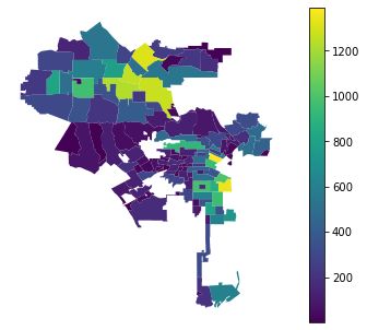
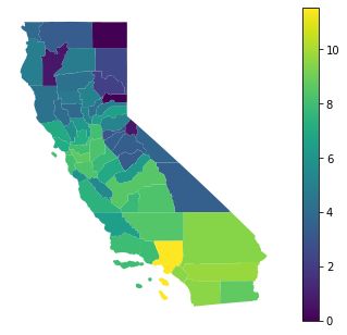
(a) LA Neighborhoods (b) California Counties

Figure 4: Cumulative COVID-19 case counts on 30 June 2020 in (a) Los Angeles
neighborhoods and (b) California counties. We plot the LA case counts on a linear
scale and the California county case counts on a (natural) logarithmic scale.

 In our case study, we use PH to analyze the spatial properties of the spread of
 COVID-19 in Los Angeles (LA) neighborhoods and California counties. In contrast
 to prior work, we use PH in a way that incorporates the underlying geographic
 structure and various spatial relationships. We consider two data sets. The first
 is a highly granular data set that consists of COVID-19 case counts in 136 LA
 neighborhoods on 30 June 2020. The second is a coarser data set that consists of
 case counts in the 58 counties of California on the same day [8]. For each data
 set, we also have geographic information in the form of a shapefile [12, 24]. We
 visualize these data sets in Figure 4.
 Let LA denote the 2D manifold that consists of the union of LA neighborhoods
 with fewer than 750 cumulative cases, and let denote the union of California
 counties with fewer than 5, 000 cumulative cases. We approximate these manifolds
 by rasterizing the associated shapefiles to obtain manifolds 0LA and 0CA . We
 show 0LA and 0CA in Figure 5. As we described in Section 2, we construct
 sequences of manifolds starting from 0LA and 0CA using level-set dynamics (1).
 We then construct a level-set filtration for each of these sequences by imposing the
 manifolds in them on a triangulation of the plane.
 In Figure 6, we show the PDs that we compute for the 1D PH of our level-set
 complexes for the two data sets. These PDs can help us identify COVID-19 hotspots.
 We define a “hotspot” to be a collection of regions — sets of neighborhoods in
 the LA data and sets of counties in the California data — in which the case count
 is higher than in the surrounding area. This notion of a hotspot is analogous to
 the political “islands” that were studied using PH in [10]. Hotspots with a case
 count that is at least as large as the threshold (750 for LA neighborhoods and
 5,000 for California counties) appear as holes in 0 , unless the hotspot is adjacent
 to the boundary of the map. The hotspots that are not adjacent to the boundary
 correspond to homology classes that are born at time 0. Note that there is not a

 6

(a) 0LA (b) 0CA

Figure 5: Initial manifolds for the level-set filtrations that we construct from data of
the spread of COVID-19. (a) The manifold 0LA is an approximation of the manifold
 LA , which consists of the union of LA neighborhoods with fewer than 750 cumulative
cases on 30 June 2020. (b) The manifold 0CA is an approximation of the surface CA ,
which consists of the union of California counties with fewer than 5, 000 cumulative
cases on 30 June 2020.

 one-to-one correspondence between hotspots and homology classes that are born
 at time 0. Some of the homology classes that are born at 0 are simply holes in
 the map (e.g., see Figure 4a), and hotspots that are adjacent to a boundary do not
 necessarily correspond to any homology class. Homology classes that are born after
 time 0 usually reflect only the geography of the regions, although they sometimes
 correspond to hotspots on the boundary of the map (much like the homology classes
 that are created by city blocks with dead ends in the Shanghai street networks). The
 PDs reflect both the number of hotspots and the sizes of the hotspots.

 5 Conclusions
 In this chapter, we discussed the importance of incorporating spatial information
 into TDA when one uses it to study spatial systems. As case studies, we computed
 PH using a level-set construction of filtered simplicial complexes on two case
 studies: city street networks in Shanghai and hotspots in the spread of COVID-19
 infections.
 In our case study of street networks in Shanghai, we illustrated that PH can cap-
 ture both topological and geometric properties of the organization of city streets.
 We also observed that the PHs of Shanghai’s street networks reflect underlying
 differences in urban planning and organization. This suggests that topological
 tools can summarize information about how humans organize themselves in space,
 although further study is necessary to fully understand what types of spatial orga-
 nization are amenable to TDA.
 In our case study of the spread of COVID-19, we showed that one can use a
 level-set filtration to study the number and sizes of COVID-19 hotspots on both a

 7

(a) LA neighborhoods (b) CA counties

Figure 6: The PDs of the level-set filtrations for COVID-19 cases in (a) LA and (b)
California.

 granular level (by considering neighborhoods in Los Angeles) and a coarse level (by
 considering counties in California). We used only case counts in our computations,
 but one can also construct level-set filtrations for the death counts, hospitalization
 counts, or other quantities. The level-set filtration is flexible, but our approach has
 important limitations. For example, we only detected hotspots with a case count
 that is above some fixed threshold. This restricts us to measuring the severity of an
 outbreak based on its geographic area. One way to address this issue is by applying
 the level-set filtration after constructing a cartogram [11], instead of directly from
 a shapefile. Additionally, the level-set filtration is unable to detect hotspots that
 occur on the boundary of a map. Addressing these limitations is part of ongoing
 work.
 Many spatial systems are also social in nature, and there are major challenges
 to overcome when studying such systems using TDA. In this chapter, we studied
 spatial systems, but it is important to point out that many spatial systems (including
 the examples in this chapter) reflect complicated social dynamics. For example,
 the Shanghai street networks have been shaped by social processes like colonial
 occupation and displacement of historical neighborhoods. Additionally, COVID-19
 is known to disproportionately affect certain communities because of a confluence
 of social factors, including who is in prison [17], where hospitals are located [19],
 and so on. The interaction between social and spatial systems is complicated and
 inseparable, and intense work is necessary to connect approaches like TDA in
 spatial systems to the social factors at play.

 Acknowledgements
 We thank the Los Angeles County Department of Public Health for providing the
 LA County data on COVID-19, and we thank Federico Battiston and Giovanni Petri
 for the invitation to write this chapter. We acknowledge support from the National
 Science Foundation (grant number 1922952) through the Algorithms for Threat
 Detection (ATD) program. MAP also acknowledges support from the National
 Science Foundation (grant number DMS-2027438) through the RAPID program.

 8

References
 [1] M. Barthelemy. Morphogenesis of Spatial Networks. Springer International
 Publishing, Cham, Switzerland, 2018.
 [2] G. Bobashev, I. Segovia-Dominguez, Y. R. Gel, J. Rineer, S. Rhea, and
 H. Sui. Geospatial forecasting of COVID-19 spread and risk of reaching
 hospital capacity. SIGSPATIAL Special, 12(2):25–32, 2020.
 [3] G. Boeing. Osmnx: New methods for acquiring, constructing, analyzing, and
 visualizing complex street networks. Computers, Environment, and Urban
 Systems, 65:126–139, 2017.
 [4] Geoff Boeing. Urban spatial order: Street network orientation, configuration,
 and entropy. Applied Network Science, 4(1):67, 2019.
 [5] M. Buchet, Y. Hiraoka, and I. Obayashi. Persistent homology and materials
 informatics. In Nanoinformatics, pages 75–95. Springer-Verlag, Heidelberg,
 Germany, 2018.
 [6] H. M. Byrne, H. A. Harrington, R. Muschel, G. Reinert, B. J. Stolz, and
 U. Tillmann. Topology characterises tumour vasculature. Mathematics Today,
 55(5):206–210, 2019.
 [7] G. Carlson. Topological methods for data modelling. Nature Reviews Physics,
 2:697–707, 2020.
 [8] USA Facts. US COVID-19 cases and deaths by state. https://usafacts.
 org/visualizations/coronavirus-covid-19-spread-map/ (1 July
 2020).
 [9] M. Feng and M. A. Porter. Spatial applications of topological data analy-
 sis: Cities, snowflakes, random structures, and spiders spinning under the
 influence. Physical Review Research, 2:033426, 2020.
[10] M. Feng and M. A. Porter. Persistent homology of geospatial data: A case
 study with voting. SIAM Review, 63(1):67–99, 2021.
[11] M. T. Gastner and M. E. J. Newman. Diffusion-based method for producing
 density-equalizing maps. Proceedings of the National Academy of Sciences
 of the United States of America, 101(20):7499–7504, 2004.
[12] Los Angeles GeoHub. LA Times neighborhood
 boundaries. https://geohub.lacity.org/datasets/
 d6c55385a0e749519f238b77135eafac_0?geometry=-120.145%
 2C33.622%2C-116.676%2C34.419 (3 June 2020).
[13] Q. Guan. Lilong housing, a traditional settlement form. https://www.
 mcgill.ca/mchg/student/lilong, 1996. M. Arch. Thesis, McGill Uni-
 versity.
[14] P. S. P. Ignacio and I. K. Darcy. Tracing patterns and shapes in remittance
 and migration networks via persistent homology. European Physical Journal
 — Data Science, 8(1):1, 2019.
[15] T. Kanagaratnam and K. Knyazeva. Demolition of Laoximen: Shanghai’s
 best link to its pre-colonial past may soon be gone. SupChina. https://
 supchina.com/2017/12/13/demolition-of-laoximen-shanghai/
 (13 December 2017).

 9

[16] L. Kanari, P. Dłotko, M. Scolamiero, R. Levi, J. Shillcock, K. Hess, and
 H. Markram. A topological representation of branching neuronal morpholo-
 gies. Neuroinformatics, 16(1):3–13, 2018.
[17] A. Nellis. The color of justice: Racial and ethnic disparity in state
 prisons. https://www.sentencingproject.org/publications/
 color-of-justice-racial-and-ethnic-disparity-in-state-prisons/
 (14 June 2016).
[18] M. E. J. Newman. Networks. Oxford University Press, Oxford, UK, 2 edition,
 2018.
[19] C. A. Nguyen, M. E. Chernew, I. Ostrer, and N. D. Beaulieu. Comparison
 of healthcare delivery systems in low- and high-income communities. The
 American Journal of Accountable Care, 7(4):11–18, 2019.
[20] World Health Organization. Coronavirus disease (COVID-19)
 pandemic. https://www.who.int/emergencies/diseases/
 novel-coronavirus-2019 (19 March 2021), 2021.
[21] S. J. Osher and R. Fedkiw. Level Set Methods and Dynamic Implicit Surfaces,
 volume 153. Springer-Verlag, Heidelberg, Germany, 2003.
[22] N. Otter, M. A. Porter, U. Tillmann, P. Grindrod, and H. A. Harrington. A
 roadmap for the computation of persistent homology. European Physical
 Journal — Data Science, 6:17, 2017.
[23] L. Papadopoulos, M. A. Porter, K. E. Daniels, and D. S. Bassett. Network
 analysis of particles and grains. Journal of Complex Networks, 6(4):485–565,
 2018.
[24] California Open Data Portal. California county boundaries.
 https://data.ca.gov/dataset/ca-geographic-boundaries/
 resource/b0007416-a325-4777-9295-368ea6b710e6 (10 September
 2019), 2019.
[25] H. Ronellenfitsch and E. Katifori. Global optimization, local adaptation,
 and the role of growth in distribution networks. Physical Review Letters,
 117(13):138301, 2016.
[26] H. Ronellenfitsch, J. Lasser, D. C. Daly, and E. Katifori. Topological phe-
 notypes constitute a new dimension in the phenotypic space of leaf venation
 networks. PLOS Computational Biology, 11(12):e1004680, 2015.
[27] B. X. Sang. Pudong: Another special economic zone in China? — An
 analysis of the special regulations and policy for Shanghai’s Pudong New
 Area. Northwestern Journal of International Law and Business, 14(1):130–
 160, 1993.
[28] A. E. Sizemore, J. E. Phillips-Cremins, R. Ghrist, and D. S. Bassett. The
 importance of the whole: Topological data analysis for the network neurosci-
 entist. Network Neuroscience, 3(3):656–673, 2019.
[29] A. Smith and V. Zavala. The Euler characteristic: A general topological
 descriptor for complex data. arXiv:2103.3144, 2021.
[30] M. Soliman, V. Lyubchich, and Y. R. Gel. Ensemble forecasting of the
 Zika space-time spread with topological data analysis. Environmetrics,
 31(7):e2629, 2020.

 10

[31] L. Speidel, H. A. Harrington, S. J. Chapman, and M. A. Porter. Topolog-
 ical data analysis of continuum percolation with disks. Physical Review E,
 98(1):012318, 2018.
[32] B. J. Stolz, J. Tanner, H. A. Harrington, and V. Nanda. Geometric anomaly
 detection in data. Proceedings of the National Academy of Sciences of the
 United States of America, 117(33):19664–19669, 2020.
[33] D. Taylor, F. Klimm, H. A. Harrington, M. Kramár, K. Mischaikow, M. A.
 Porter, and P. J. Mucha. Topological data analysis of contagion maps for ex-
 amining spreading processes on networks. Nature Communications, 6(7723),
 2015.
[34] C. M. Topaz, L. Ziegelmeier, and T. Halverson. Topological data analysis of
 biological aggregation models. PLOS ONE, 10(5):e0126383, 05 2015.
[35] A. Vespignani, H. Tian, C. Dye, J. O. Lloyd-Smith, R. M. Eggo, M. Shrestha,
 S. V. Scarpino, B. Gutierrez, M. U. G. Kraemer, J. Wu, K. Leung, and G. M.
 Leung. Modelling COVID-19. Nature Reviews Physics, 2(279–281), 2020.
[36] M. Walsh. In old Shanghai, a last spring festival before the bulldozers.
 https://www.sixthtone.com/news/1003537/in-old-shanghai%
 2C-a-last-spring-festival-before-the-bulldozers (4 February
 2019).
[37] Y. M. Yeung and Y. w. Sung, editors. Shanghai: Transformation and Mod-
 ernization Under China’s Open Policy. Chinese University of Hong Kong
 Press, Hong Kong, 1996.
[38] S. Zhu, A. Bukharin, L. Xie, M. Santillana, S. Yang, and Y. Xie. High-
 resolution spatio-temporal model for county-level COVID-19 activity in the
 U.S., 2020. arXiv:2009.07356.

 11