Whistler waves produced by monochromatic currents in the low nighttime ionosphere
←
→
Page content transcription
If your browser does not render page correctly, please read the page content below
Ann. Geophys., 39, 479–486, 2021
https://doi.org/10.5194/angeo-39-479-2021
© Author(s) 2021. This work is distributed under
the Creative Commons Attribution 4.0 License.

Whistler waves produced by monochromatic currents
in the low nighttime ionosphere
Vera G. Mizonova1,2 and Peter A. Bespalov3
1 Nizhny   Novgorod State Technical University, Department of General and Nuclear Physics, Nizhny Novgorod, Russia
2 National  Research University Higher School of Economics, Department of Mathematics, Nizhny Novgorod, Russia
3 Institute of Applied Physics RAS, Department of Astrophysics and Space Plasma Physics, Nizhny Novgorod, Russia

Correspondence: Peter A. Bespalov (pbespalov@mail.ru)

Received: 19 July 2020 – Discussion started: 26 August 2020
Revised: 4 May 2021 – Accepted: 12 May 2021 – Published: 9 June 2021

Abstract. We use a full-wave approach to find the field of            Several numerical methods have been developed for cal-
monochromatic whistler waves, which are excited and prop-          culating whistler wave fields in the Earth’s ionosphere (Pit-
agating in the low nighttime ionosphere. The source current        teway, 1965; Wait, 1970; Bossy, 1979; Nygre’n, 1982; Bud-
is located in the horizontal plane and can have arbitrary finite   den, 1985; Nagano et al., 1994; Yagitani et al., 1994; Sha-
distribution over horizontal coordinates. The ground-based         lashov and Gospodchikov, 2011). One of the main difficul-
horizontal magnetic field and electric field at 125 km are cal-    ties is numerical instabilities caused by a large imaginary
culated. The character of wave polarization on the ground          part of the vertical wave number. General full-wave analy-
surface is investigated. The proportion in which source en-        sis, including the problem of numerical “swamping” of the
ergy supplies the Earth–ionosphere waveguide or flows up-          evanescent wave solutions, was performed, for example, by
ward can be adjusted by distribution of the source current.        Nygre’n (1982), Nagano et al. (1994), and Budden (1985). A
Received results are important for the analysis of ELF/VLF         traditional approach in full-wave analysis is to divide a strat-
emission phenomena observed both on the satellites and on          ified ionosphere into a number of thin horizontal and homo-
the ground.                                                        geneous slabs and then connect the solutions in each slab by
                                                                   applying the boundary conditions. Such a technique has been
                                                                   used by Yagitani et al. (1994) to study ELF/VLF propagation
                                                                   from an infinitesimal dipole source located in the lower iono-
                                                                   sphere. The idea of recursive calculation of mode amplitudes
1   Introduction                                                   was developed and used for an arbitrary configuration of the
                                                                   radiating sources by Lehtinen and Inan (2008). Nevertheless,
ELF/VLF waves, which propagate in the ionosphere in                finding fields created by both natural and artificial ELF/VLF
whistler mode, are an important part of the ionosphere dy-         radiating sources is still very relevant.
namics. Such waves can be emitted by various natural phe-             In this paper, we use numerical methods to find the field of
nomena such as atmospheric lightning discharges and vol-           ELF/VLF waves, which have been produced in a low night-
                                                                                                                                      AnGeo Communicates

canic eruptions, magnetospheric chorus and hiss. Artificial        time ionosphere. On the one hand, significant inhomogeneity
ELF/VLF waves have been produced by ground-based trans-            of plasma parameters, strong wave mode attenuation and ef-
mitters and by modulated high-frequency (HF) heating of the        fect of wave mode transformation (for example, whistler to
ionosphere current system responsible for Sq variations or         vacuum electromagnetic) in the low-altitude nighttime iono-
the auroral electrojet, which is by now a well-known tech-         sphere make the problem considered difficult enough and
nique. ELF/VLF waves modulated by the HAARP heating                fundamentally important. On the other hand, it has practical
facility can be injected in the Earth–ionosphere waveguide         significance, as an example, for interpretation of numerous
as far as 4400 km (Moore et al., 2007) and also into space
(Inan et al., 2004).

Published by Copernicus Publications on behalf of the European Geosciences Union.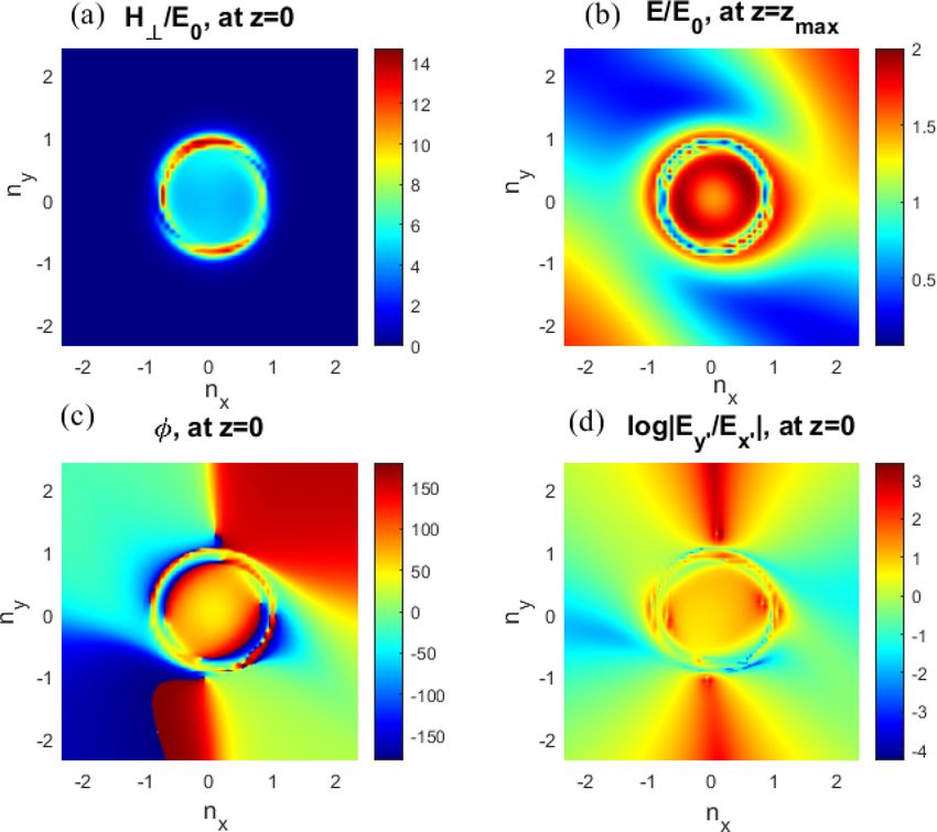
480 V. G. Mizonova and P. A. Pespalov: Whistler waves produced by currents in the ionosphere
experimental results on HF heating which modulate natural tions
ionospheric currents at altitudes of 60–100 km.
In calculations, we use a technique known as the two-point ∇ × H = Z0 j − ik0 ε̂E,
boundary-value problem for ordinary differential equations ∇ × E = ik0 H , (4)
(Kierzenka and Shampine, 2001). Using this technique in
early work (Bespalov and Mizonova, 2017; Bespalov et al., where c is the speed of light in free space and ε̂ is the per-
2018) has provided numerically stable solutions of a com- mittivity tensor, which yield a set of four equations for the
plete system of wave equations for arbitrary altitude profiles horizontal components E ⊥ (n⊥ , z), H ⊥ (n⊥ , z) (in a case of
of plasma parameters and in the stratified ionosphere for ar- a source-free medium, see, e.g., Budden, 1985, Bespalov et
bitrary angles of wave incidence from above. Here, we find al., 2018, and Mizonova, 2019)
a wave field created by a monochromatic source current lo-
cated in the low night ionosphere. We examine the influence dF /dz = M̂F + Z0 I δ(z − zs ). (5)
of peculiarities of current distribution on the proportion in
Here we have taken into account that the horizontal refractive
which source energy supplies the Earth–ionosphere waveg-
index of the wave propagating through the stratified medium
uide or flows upward. As an example of calculations, we use
is conserved due to Snell’s law. In Eq. (5) F (n⊥ , z) and
current distributions similar to those simulated by HF heat-
I (n⊥ , z) are four-component column vectors
ing of the auroral electrojet (Payne et al., 2007). The obtained
results are important for analysis of the ELF/VLF emission
Ex
nx Jz /εzz
phenomena observed both in the ground-based observatories Ey ny Jz /εzz
and onboard satellites. F = Hx , I = Jy − Jz (η − ε) sin 2ϑ/2εzz . (6)
Hy −Jx + Jz ig sin ϑ/εzz
2 Basic equations
M̂ is a matrix of which the elements mij are expressed in
We consider a whistler wave which is excited and propa- terms of components of the transverse wave vector k ⊥ =
gating in the layer 0 ≤ z ≤ zmax of the non-homogeneous k0 n⊥ , and ε, η, and g are elements of the permittivity tensor
stratified ionosphere. We choose a coordinate system with which depends on the z coordinate (Bespalov and Mizonova,
a vertical upward z axis and x and y axes in the horizon- 2017; Bespalov et al., 2018), εzz = εsin2 ϑ + ηcos2 ϑ.
tal plane, suppose that plasma parameters depend on coordi- To solve the system in Eq. (5), in Eq. (6) we define four
nate z, plane z = 0 corresponds to the ground surface, above boundary conditions. We write two of them on the plane z =
the boundary z = zmax ionosphere plasma is close to homo- 0 assuming the ground surface to be perfectly conductive:
geneous, and the ambient magnetic field B 0 belongs to the
Ex (z = 0) = 0, Ey (z = 0) = 0. (7)
y–z plane and is inclined at an angle ϑ to the z axis. We as-
sume that external currents have monochromatic dependence
We write two other conditions on the plane z = zmax exclud-
on time and flow in the source plane z = zs :
ing wave energy coming from above. To clarify them, we ex-
press the field vector column F above the boundary z = zmax
j (r ⊥ , z, t) = J (r ⊥ ) δ (z − zs ) e−iωt . (1)
as the sum of four wave modes
At first, we use the Fourier composition of the source current 4
X
density over the horizontal coordinates, F (z) = Aj P j exp ikzj (z − zmax ) . (8)
Z j =1
J (n⊥ , z) = J (r ⊥ , z) e−ik0 n⊥ r ⊥ k02 dr ⊥ , (2)
Here Aj = const, kzj are four roots of the local dispersion re-
lation and P j are four corresponding local polarization vec-
and wave electric and magnetic fields at each altitude tors. We mention that values kzj and vectors P j are the so-
Z lutions of Eqs. (5) and (8) for homogeneous plasma without
E (n⊥ , z) = E (r ⊥ , z) e−ik0 n⊥ r ⊥ k02 dr ⊥ , sources. Assuming that indices 2 and 4 correspond to coming
Z from above-propagating and non-propagating wave modes
(imaginary parts of kz2 and kz4 are negative), we write
H (n⊥ , z) = H (r ⊥ , z) e−ik0 n⊥ r ⊥ k02 dr ⊥ , (3)
A2 = 0, A4 = 0. (9)
and find field amplitudes E(n⊥ , z), H (n⊥ , z) correspond-
ing to the horizontal wave vector component k ⊥ = k0 n⊥ , Solving the set of Eq. (5) with known source current den-
k0 = ω/c. Here we use SI units for E and modified
√ units sity Eq. (6) and boundary conditions Eqs. (7) and (9), we can
for H = Z0 H SI (Budden, 1985), where Z0 = µ0 /ε0 is the find the field of the plane wave with horizontal wave vec-
impedance of free space. Then we write the Maxwell equa- tor k ⊥ = k0 n⊥ in the layer 0 < z < zmax . Then, we use the
Ann. Geophys., 39, 479–486, 2021 https://doi.org/10.5194/angeo-39-479-2021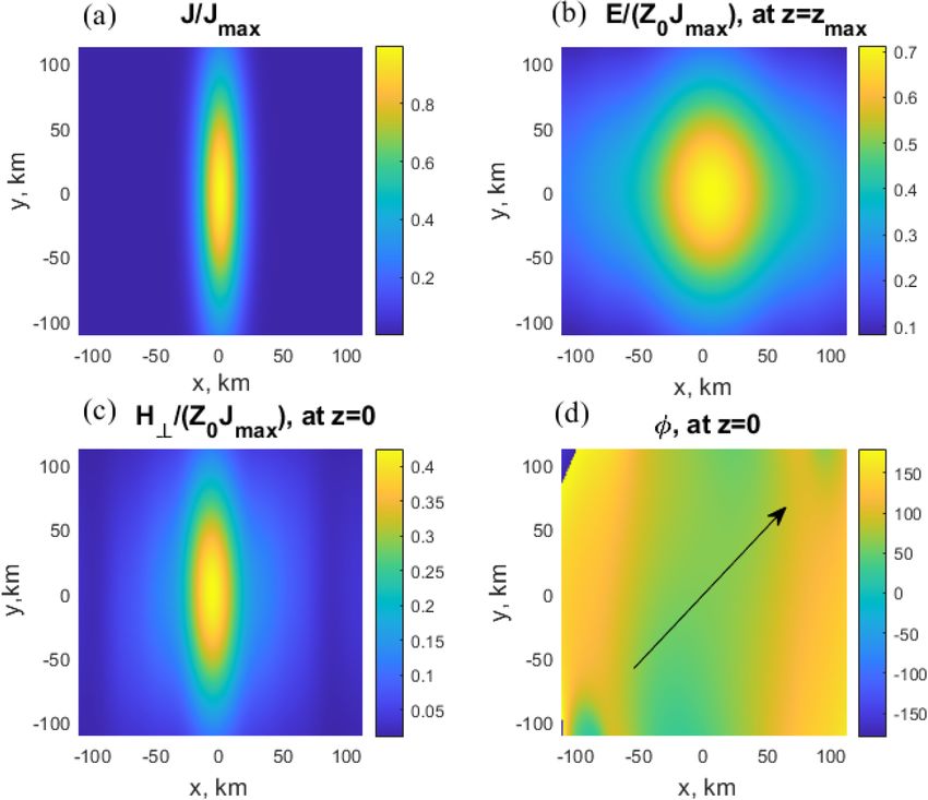
V. G. Mizonova and P. A. Pespalov: Whistler waves produced by currents in the ionosphere                                              481

inverse transform                                                  particular, the fields on the ground surface can be expressed
             Z                                                     as
                                      dn⊥
E (r ⊥ , z) = E (n⊥ , z) eik0 n⊥ r ⊥        ,              (10)                    q
                                     (2π )2                        H⊥ (z = 0) = |Hx (z = 0)|2 + Hy (z = 0) ,
                                                                                                                  2
             Z
                                       dn⊥
H (r ⊥ , z) = H (n⊥ , z) eik0 n⊥ r ⊥

                                             ,             (11)                              ny
                                      (2π )2                       Ey (z = 0) = sin ϑ −
                                                                      0                          cos ϑ nx Hy (z = 0) −
                                                                                             n0z

to calculate the total field.                                                   2 cos ϑ

                                                                   − 1 − ny               + ny sin ϑ Hx (z = 0) ,
                                                                                    n0z
3   Description of the solution algorithm                                         1 − n2x              nx ny
                                                                   Ex 0 (z = 0) =         Hy (z = 0) +       Hx (z = 0) ,   (16)
                                                                                    n0z                 n0z
We take into account that out of the plane z = zs , the source                   q
current density Eq. (6) is equal to zero, so Eq. (5) becomes       where n0z = 1 − n2⊥ , Ex 0 ,y 0 are electric strength compo-
                                                                   nents of the incident wave in the coordinate system with the
dF /dz = M̂F .                                             (12)    z0 axis along the ambient magnetic field. The wave polariza-
                                                                   tion near the ground surface is determined by
To solve Eq. (11) in layers 0 ≤ z < zs and zs < z ≤ zmax , we
apply packaged solver MATLAB bvp4c and use a method                5 = Ey 0 (z = 0) /Ex 0 (z = 0) .                                   (17)
known as the two-point boundary-value problem for ordi-
nary differential equations (Kierzenka and Shampine, 2001).        The electric field at the altitude z = zmax can be expressed as
The solver solution starts with an initial guess supplied at an
                                                                   E (z = zmax ) =
initial mesh point and changes step size to get the specified          q
accuracy.                                                          =
                                                                                                              2
                                                                           |Ex (z = zmax )|2 + Ey (z = zmax ) + |Ez (z = zmax )|2 .   (18)
   At first we find two linearly independent solutions F 1 and
F 2 of Eq. (11) in the layer 0 ≤ z < zs completing the bound-      The coordinate dependence of the wave field can be found
ary condition Eq. (7) on the plane z = 0 for arbitrary condi-      from the inverse Fourier transform Eq. (10). The vertical en-
tions on the plane z = zs − 0. For example, we use four con-       ergy flux (Poynting vector) is
ditions Ex (z = 0) = 0, Ey (z = 0) = 0, Ex (z = zs − 0) = E,
                                                                   Sz = (2Z0 )−1 Re E ∗⊥ , H ⊥ z ,

and Ey (z = zs − 0) = 0 for the solution F 1 and four con-                                                                  (19)
ditions Ex (z = 0) = 0, Ey (z = 0) = 0, Ex (z = zs − 0) = 0,       and the total power of the source is
and Ey (z = zs − 0) = E for the solution F 2 , where E is                    Z
constant. Then we write the general solution in the layer               1
                                                                   P = Re         jx Ex∗ (z = zs ) + jy Ey∗ (z = zs ) dxdy.           (20)
0 ≤ z ≤ zs as the sum                                                   2

F = aF 1 + bF 2 .                                          (13)    Now we present the results of the numerically computed so-
                                                                   lution of the set Eqs. (5) and (6) under model conditions for
Similarly, we find two linearly independent solutions F ∗1 and     the nighttime ionosphere.
F ∗2 of Eq. (11) in the upper layer zs < z ≤ zmax completing
the boundary condition Eq. (9) on the plane z = zmax . By
                                                                   4   The ionosphere data and calculation results
arbitrary conditions on the plane z = zs + 0, we have A2 =
0, A4 = 0, Ex (z = zs + 0) = E, and Ey (z = zs + 0) = 0 and        In the calculations, we use the altitude profiles of the
A2 = 0, A4 = 0, Ex (z = zs + 0) = 0, and Ey (z = zs + 0) =         plasma density shown in Fig. 1a and the collision frequen-
E, respectively. We write the general solution in the layer        cies between charged and neutral particles shown in Fig.
zs < z ≤ zmax as the sum                                           1b. The plasma density data are taken from International
                                                                   Reference Ionosphere (Bilitza and Reinisch, 2007), avail-
F = a ∗ F ∗1 + b∗ F ∗2 .                                   (14)
                                                                   able from CCMC at https://ccmc.gsfc.nasa.gov/modelweb/
Integrating Eq. (5) over the z coordinate in a narrow layer        models/iri2016_vitmo.php (last access: 28 April 2021), and
(zs − 0, zs + 0), we find a condition connecting solutions         correspond to 680 N, 250 E; 4 September 2019, 00:30 LT. The
Eqs. (12) and (13):                                                collision frequency data are taken from the book of Gurevich
                                                                   and Shvarcburg (1973). The angle of magnetic field inclina-
F (z = zs + 0) − F (z = zs − 0) = Z0 I .                   (15)    tion with respect to the axis z is equal to ϑ = 1680 . We use
                                                                   the value zmax = 125 km as the upper boundary of the solu-
That condition yields four algebraic equations for the coeffi-     tion. At this altitude a typical spatial scale of plasma inhomo-
cients a, a ∗ , b, and b∗ . Thus, finding those coefficients, we   geneity exceeds 70 km, and it is much more than the wave-
obtain the wave field F Eq. (6) in the layer 0 ≤ z ≤ zmax . In     length, which in the considered case is on order 20 to 25 km.

https://doi.org/10.5194/angeo-39-479-2021                                                          Ann. Geophys., 39, 479–486, 2021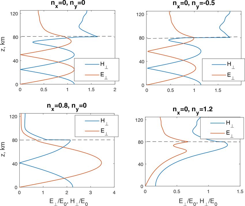
482 V. G. Mizonova and P. A. Pespalov: Whistler waves produced by currents in the ionosphere
Figure 1. Nighttime ionosphere model: (a) the electron plasma den-
sity and (b) the collision frequency between electron and neutral Figure 2. Fields in the z = 0 plane: (a) characteristic horizon-
particles (solid line) and collision frequency between ion and neu- tal sizes of the horizontal magnetic field, (b) the electric field
tral particles (dashed line). atthe height z = 125 km, (c) the polarization ellipse parameters
φ Ey 0 = Ex 0 eiφ , and (d) log Ey 0 /Ex 0 .
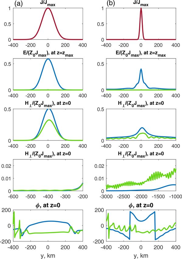
As an example, we calculate the fields created by varying at
frequency 3 kHz and flowing at the altitude zs = 80 km hori-
electric and magnetic fields corresponding to different
zontal current.
horizontal refractive indices are presented in Fig. 3. The
We assume that currents occupy a volume which has a
level z = zs of the source action is marked by a dotted
shape of a horizontal pancake and use for calculations a
line. Figure 4 shows contour maps of fields created by
Gaussian distribution over x and y coordinates
horizontal currents (20) with characteristic horizontal sizes
Lx ' 12 km, Ly ' 70 km and equal x and y components
J (r ⊥ ) = Jmax exp −x 2 /2L2x − y 2 /2L2y . (21)
Jx = Jy current density (Fig. 4a), electric field at altitude
The corresponding current distribution Eq. (2) in z = zmax (Fig. 4b), horizontal magnetic field on ground sur-
Fourier space is also Gaussian and face z = 0 (Fig. 4c) and polarization parameter φ (Fig. 4d).
has a form Current density is normalized by the value Jmax , both
J (n⊥ ) = J0 exp −k02 L2x n2x /2 − k02 L2y n2y /2 , where
electric and magnetic fields are normalized by the value
J0 = 2π k02 Lx Ly Jmax . We calculate the wave field in Z0 Jmax , and the arrow shows the current direction. Exam-
N = 1000 points with steps and then use inverse fast Fourier ples of ground-based horizontal magnetic field and electric
transform (Cooley and Tukey, 1965) to find its coordinate field at altitude z = zmax corresponding to the coordinate
dependence. We present the results of field calculation in x = 0, characteristic horizontal sizes of source Ly ' 70 km,
Fourier space (Figs. 2–3) and in coordinate space (Fig. 4). Ly ' 12 km and different distributions of Jx,y are presented
The dependences of amplitude of horizontal magnetic field in Fig. 5.
H⊥ (nx , ny )/E0 on ground surface z = 0 and amplitude
of electric field E(nx , ny )/E0 at altitude z = zmax are
presented in Fig. 2a, b. The field values are normalized by 5 Discussion
the value E0 = Z0 J0 . Polarization ellipse parameters φ,
Ey 0 = Ex 0 e−iφ , and log Ey 0 /Ex 0 are presented in Fig. 2c, We use a full-wave approach to find the field of monochro-
d. Positive values of phase φ correspond to right-hand matic whistler waves which are excited and propagating
polarization, typical for whistler waves, and negative values at night in the strongly inhomogeneous low ionosphere. A
of phase φ correspond to left-hand polarization. Positive source current is assumed to be located in the horizontal
values of parameter log Ey 0 /Ex 0 mean that the polarization plane and to have in this plane an arbitrary finite-space dis-
ellipse is elongated predominantly along the y axis, and tribution. At first, we consider a plane wave with the hori-
negative values of parameter log Ey 0 /Ex 0 mean that the zontal components of the refractive index n⊥ generated by
polarization ellipse is elongated predominantly along the the current J (r ⊥ ) ∼ eik0 n⊥ r ⊥ . The set of wave equations in
x axis. Examples of altitude dependences of normalized the layer 0 < z < zmax for each n⊥ component is completed
Ann. Geophys., 39, 479–486, 2021 https://doi.org/10.5194/angeo-39-479-2021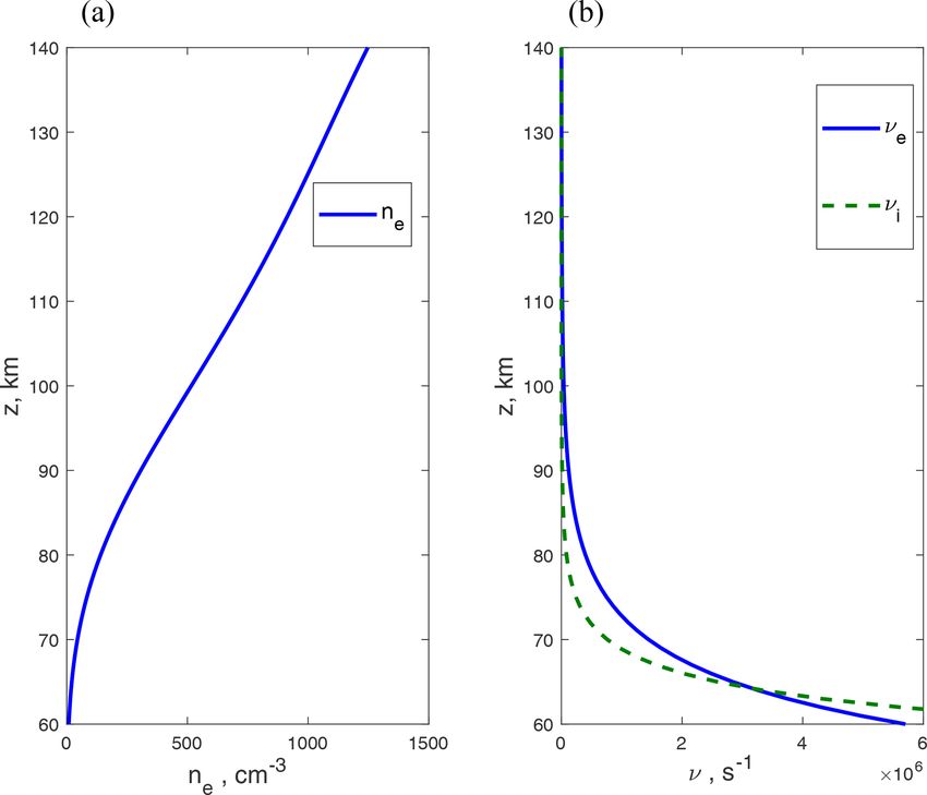
V. G. Mizonova and P. A. Pespalov: Whistler waves produced by currents in the ionosphere                                             483

Figure 3. Altitude dependences of the amplitudes of horizontal
                                                                   Figure 4. Source currents and field space distributions: (a) space
electric and magnetic fields.
                                                                   distributions of source currents, (b) the electric field at z = 125 km,
                                                                   (c) the horizontal magnetic field at z = 0, and (d) the polarization
                                                                   ellipse parameters φ, Ey 0 = Ex 0 e−iφ at z = 0.
by boundary conditions assuming a perfect conductivity of
the ground surface and excluding wave energy coming on
the upper boundary z = zmax from above. The mathemati-
cal method known as the two-point boundary-value problem
for ordinary differential equations (Kierzenka and Shampine,
2001) is applied to find the solutions of wave equations above
and below the source plane. Then we connect these solutions
using source current distribution. When the dependencies of
source current and wave field in n⊥ space are finite functions
with discretized values, the fast Fourier transform algorithm
can be used for numerical calculations. Inverse fast Fourier
transform yields space dependence of the wave field.
   As an example, we calculate the fields created by vary-
ing at a frequency of 3 kHz and flowing at zs = 80 km hor-
izontal current, with a Gaussian distribution of source cur-
rent density over x and y coordinates. We mention that the
model of a plane source current can also be effective in a
more general case of a current layer with small thickness
1z  λz ∼ 60 km. The ground-based horizontal magnetic
field and the electric field at 125 km are calculated in both
Fourier (nx , ny ) and coordinate (x, y) spaces, since a wave
can achieve the ground surface in penetrating mode in case
n⊥ ≤ 1. The magnetic field H⊥ (n⊥ , z = 0) is noticeably non-
zero for Fourier components with n⊥ < 1 and is practically
equal to zero for Fourier components with n⊥  1. Waves
with n⊥ < 1 are right-hand-polarized (see Fig. 2c), which is
typical for whistlers. However, if the horizontal component        Figure 5. Current density (red line) and field space distributions at
of the refractive index has an order of unit, then the mag-        x = 0 for two different ratios Jy /Jx , outlined by green (Jy /Jx = 1)
                                                                   and blue (Jy /Jx ' −i) colors. Left plot column (a) corresponds to
netic field H⊥ (n⊥ , z = 0) can increase by 2 or 3 times (see
                                                                   the Ly = 70 km ≥ 1/k0 source scale and right plot column (b) cor-
Fig. 2a). The polarization parameter φ of such components
                                                                   responds to the Ly = 12 km ≤ 1/k0 source scale.
can be negative, similarly to the left-hand-polarized waves
(see Fig. 2c). A typical size of the spot and a character of po-
larization of the ground-based magnetic field H⊥ (r⊥ , z = 0)

https://doi.org/10.5194/angeo-39-479-2021                                                       Ann. Geophys., 39, 479–486, 2021
484 V. G. Mizonova and P. A. Pespalov: Whistler waves produced by currents in the ionosphere depend on the source distribution. If the horizontal size of ionosphere waveguide or flows upward mainly depends on the radiating currents exceeds a value L ≥ 1/k0 ∼ 15 km (for polarization of the source current. the wave of frequency 3 kHz), then the Fourier components If the horizontal size of radiating currents is small enough, with n⊥ ≤ 1 dominate in the total field. In that case, the L ≤ 1/k0 , a ground-based magnetic field can be noticeably magnetic field H⊥ (r⊥ , z = 0) is predominantly localized un- non-zero far (a few thousand kilometers) from the source der the source. If the horizontal size of radiating currents (see Fig. 5b). Propagation of modulated ELF/VLF signals is small enough L ≤ 1/k0 , then Fourier components n⊥ ∼ 1 in the Earth–ionosphere waveguide far from the source and can make a notable contribution to the total field. The mag- also into space (Inan et al., 2004) is observed experimen- netic field H⊥ (r⊥ , z = 0) occupies a spot ∼ 1/k0 but can tally. The HAARP heating facility in Gakona, Alaska, injects sometimes be registered far from the source (see Figs. 4c, ELF/VLF waves in the Earth–ionosphere waveguide as far as 5b). The field above the source is determined by both direct 4400 km (Moore et al., 2007). radiation from the source and the reflected radiation. Because The current distributions used as an example in our cal- of the effective night reflection of ELF/VLF waves, a spot of culation and presented in Fig. 4 can be similar to electro- the electric field at 125 km can exceed the size of the source jet currents modulated in the D region by the HAARP HF by several times (Fig. 4b). heating facility (Keskinen and Rowland, 2006; Payne et al., At altitudes of source and above, the two ELF/VLF 2007). For example, according to data collected during an wave modes Eq. (8) are weakly damped and have right- experimental campaign run in April 2003 and results of nu- hand polarization, and another two modes are evanescent merical simulations (Payne et al., 2007; Lehtinen and Inan, and have left-hand polarization. At altitudes ∼ 60–70 km 2008), the maximum change in modulated conductivity oc- and below all four modes transform into vacuum elec- cupies approximately 10 km over the height and occurs at tromagnetic ones. Source currents can excite both right- altitude ∼ 80 km. Pedersen and Hall conductivities approx- hand- and left-hand-polarized modes. Hence, current dis- imately coincide, so if the ambient electrojet field is directed tribution properties specify field distribution, field polariza- along the x axis, then jx ≈ jy . The maximum surface den- tion, and proportion in which source energy supplies the sity of modulated currents Eq. (1) has an order Jmax ∼ 10−6 – Earth–ionosphere waveguide or flows upward. As an exam- 10−5 A m−1 . Using in our calculations the magnitude of cur- ple, Figs. 5a, b show coordinate dependencies of source den- rent density Jmax ∼ 5 · 10−6 A m−1 yields the total power of sity, fields E (x = 0, y, z = 0), H⊥ (x = 0, y, z = 0) and po- the source ∼ 36 W, the ground-based horizontal magnetic larization parameter φ in cases of large Ly = 70 km ≥ 1/k0 field under the source B⊥ ∼ 1 pT, and the electric field at the (a) and small Ly = 12 km ≤ 1/k0 (b) sources for two differ- altitude of 125 km above the source E ∼ 400 µV m−1 . The ent ratios Jy /Jx in distribution (20), outlined by green and magnitude of the magnetic field is similar to the field mea- blue colors. In the first case of ratio Jy /Jx = 1 (blue lines on sured at VLF sites in the immediate vicinity of the HAARP the plots), source currents excite predominantly right-hand- heating facility (Payne et al., 2007) and calculated by Lehti- polarized modes. So the polarization parameter at z = 0 is nen and Inan (2008). The maximum vertical energy flux mainly positive under the source. Approximately 50 %–60 % (Poynting vector) at the altitude of 125 km is ∼ 3.2 nW m−2 , of the source energy is carried upward, 30 %–40 % is ad- and total power is ∼ 17 W. About half of the source energy sorbed, and about 10 % is supplied to the Earth–ionosphere is carried upward, approximately 20 % of the energy is sup- waveguide. This can be useful for modification processes plied to the Earth–ionosphere waveguide, and approximately in the plasma magnetic trap (Bespalov and Trakhtengerts, 30 % of the energy is absorbed. 1986). Of course, the electromagnetic ELF/VLF radiation of ionospheric currents themselves is not sufficient for a no- ticeable modification of the Earth’s electron radiation belts. 6 Conclusions However, under quiet conditions in the nighttime magneto- sphere, these emissions can ensure the radiation belt transi- We find a field of monochromatic whistler waves which are tion through the threshold of the cyclotron instability. This excited and propagating in the low nighttime ionosphere. Us- process can be accompanied by a significant precipitation of ing a MATLAB boundary-value problem solver enables us energetic electrons into the ionosphere and other geophysical to find numerically stable solutions of a full set of the wave manifestations. equations applying to conditions of an inhomogeneous iono- In the second case of ratio Jy /Jx ' −i ratio (green lines sphere at altitudes below 125 km. Above this altitude the on the plots), source currents excite predominantly left-hand- ionosphere plasma is slightly inhomogeneous, and hence ap- polarized modes. Respectively, the polarization parameter at proximate methods are suitable. As an example, this calcu- z = 0 becomes predominantly negative. In that case, regard- lation technique is applied to the problem of ELF/VLF wave less of source size, approximately 10 %–12 % of the energy is radiation from modulated HF-heated electrojet currents. At supplied to the Earth–ionosphere waveguide, and about 90 % first we consider a plane wave with a known horizontal com- is absorbed and not carrying upward to the magnetosphere. ponent of the refractive index, find a wave field, and analyze The proportion in which source energy supplies the Earth– a character of wave polarization on the ground surface. Then Ann. Geophys., 39, 479–486, 2021 https://doi.org/10.5194/angeo-39-479-2021
V. G. Mizonova and P. A. Pespalov: Whistler waves produced by currents in the ionosphere                                                  485

we use an inverse fast Fourier transform to find a total field,          Bespalov, P. A., Mizonova V. G., and Savina, O. N.: Re-
get the dependencies of a wave field at 0 and 125 km, and                   flection from and transmission through the ionosphere of
analyze the type of wave polarization on the ground surface.                VLF electromagnetic waves incident from the mid-latitude
The proportion in which source energy supplies the Earth–                   magnetosphere, J. Atmos. Sol.-Terr. Phys., 175, 40–48,
ionosphere waveguide, absorbs or flows upward depends on                    https://doi.org/10.1016/j.jastp.2018.04.018, 2018.
                                                                         Bilitza, D. and Reinisch, B.: International reference ionosphere: im-
the altitude profile of the ionosphere plasma. Besides, the
                                                                            provements and new parameters, J. Adv. Space Res., 42, 599–
spatial distribution of radiating energy can be regulated by                609, https://doi.org/10.1029/2007SW000359, 2007.
modulated currents. Depending on their properties, radiat-               Bossy, L.: Wave propagation in stratified anisotropic media, J. Geo-
ing energy can predominantly flow into space or inject into                 phys., 46, 1–14, 1979.
the Earth–ionosphere waveguide far from the source. The ob-              Budden, K. G.: The propagation of radio waves: the theory of ra-
tained values are in good agreement with ground and satellite               dio waves of low power in the ionosphere and magnetosphere,
observations and known calculation results. Using a model of                Cambridge Univ. Press, Cambridge, 1985.
the plane horizontal source, currents can be generalized for             CCMC (Community Coordinated Modeling Center): ModelWeb
the arbitrary altitude source distribution.                                 Catalogue and Archive, available at: https://ccmc.gsfc.nasa.
                                                                            gov/modelweb/models/iri2016_vitmo.php, last access: 28 April
                                                                            2021.
Data availability. The paper is theoretical, and no new experi-          Cooley, W. and Tukey, J. W. I.: An algorithm for the machine cal-
mental data are used. The data are taken from the International             culation of complex Fourier series, Math. Comp., 19, 297–301,
Reference Ionosphere model (Bilitza and Reinisch, 2007) (https://           https://doi.org/10.1090/S0025-5718-1965-0178586-1, 1965.
ccmc.gsfc.nasa.gov/modelweb/models/iri2016_vitmo.php, CCMC,              Gurevich, A. V. and Shvarcburg, A. B.: Nonlinear theory of radio
2021). All figures are obtained from numerical calculation in MAT-          wave propagation in the ionosphere, Nauka, Moscow, 1973 (in
LAB codes.                                                                  Russian).
                                                                         Inan, U. S., Golkowski, M., Carpenter, D. L., Reddell, N., Moore,
                                                                            R. C., Bell, T. F., Paschal, E., Kossey, P., Kennedy, E., and Meth,
                                                                            S. Z.: Multihop: Whistler-mode ELF/VLF signals and triggered
Author contributions. VGM produced the calculations, analyzed
                                                                            emissions excited by the HAARP HF heater, Geophys. Res. Lett.,
results, and wrote the paper. PAB proposed the problem, discussed
                                                                            31, L24805, https://https://doi.org/10.1029/2004GL021647,
results, and wrote the paper.
                                                                            2004.
                                                                         Keskinen, M. J. and Rowland, H. L.: Magnetospheric effects from
                                                                            man-made ELF/VLF modulation of the auroral electrojet, Radio
Competing interests. The authors declare that they have no conflict         Sci., 41, RS1006, https://https://doi.org/10.1029/2005RS003274,
of interest.                                                                2006.
                                                                         Kierzenka, J. and Shampine, L. F.: A BVP Solver based on Resid-
                                                                            ual Control and the MATLAB PSE, ACM TOMS, 27, 299–316,
Acknowledgements. The work (Sects. 2–4) is supported by RFBR                2001.
grant no. 20-02-00206A. The work of Peter A. Bespalov (Sects. 1,         Lehtinen, N. G. and Inan, U. S.: Radiation of ELF/VLF waves by
5, and 6) is supported by RSF grant no. 20-12-00268. The numerical          harmonically varying currents into a stratified ionosphere with
calculations were performed as part of the State Assignment of the          application to radiation by a modulated electrojet, J. Geophys.
Institute of Applied Physics RAS, project no. 0030-2021-0002.               Res., 113, A06301, https://doi.org/10.1029/2007JA012911,
                                                                            2008.
                                                                         Mizonova, V. G.: Matrix Algorithm of Approximate So-
Financial support. This research has been supported by the RSF              lution of Wave Equations in Inhomogeneous Mag-
(grant no. 20-12-00268).                                                    netoactive Plasma, Plasma Phys. Rep., 45, 777–785,
                                                                            https://doi.org/10.1134/S1063780X190700802019, 2019.
                                                                         Moore, R. C., Inan, U. S., Bell, T. F., and Kennedy, E. J.: ELF waves
Review statement. This paper was edited by Dalia Buresova and               generated by modulated HF heating of the auroralelectrojet and
reviewed by three anonymous referees.                                       observed at a ground distance of 4400 km, J. Geophys. Res., 112,
                                                                            A05309, https://https://doi.org/10.1029/2006JA012063, 2007.
                                                                         Nagano, I., Miyamura, K., Yagitani, S., Kimura, I., Okada, T.,
                                                                            Hashimoto, K., and Wong, A. Y.: Full wave calculation method
                                                                            of VLF wave radiated from a dipole antenna in the iono-
References                                                                  sphere – analysis of joint experiment by HIPAS and Ake-
                                                                            bono satellite, Electr. Commun. Jpn. Commun., 77, 59–71,
Bespalov, P. A. and Mizonova, V.: Propagation of a whistler wave            https://doi.org/10.1002/ecja.4410771106, 1994.
  incident from above on the lower nighttime ionosphere, Ann.            Nygre’n, T.: A method of full wave analysis with improved stability,
  Geophys., 35, 671–675, https://doi.org/10.5194/angeo-35-671-              Planet. Space Sci., 30, 427–430, https://doi.org/10.1016/0032-
  2017, 2017.                                                               0633(82)90048-4, 1982.
Bespalov, P. A. and Trakhtengerts, V. Y.: Cyclotron instability of the
  Earth radiation belts, Rev. Plasma Phys., 10, 155–292, 1986.

https://doi.org/10.5194/angeo-39-479-2021                                                            Ann. Geophys., 39, 479–486, 2021
486 V. G. Mizonova and P. A. Pespalov: Whistler waves produced by currents in the ionosphere
Payne, J. A., Inan, U. S., Foust, F. R., Chevalier, T. W., and Bell, T. Shalashov, A. G. and Gospodchikov, E. D.: Impedance tech-
F.: HF modulated ionospheric currents, Geophys. Res. Lett., 34, nique for modeling electromagnetic wave propagation in
L23101, http://https://doi.org/10.1029/2007GL031724, 2007. anisotropic and gyrotropic media, Physics-Uspekhi, 54, 145–
Pitteway, M. L. V.: The numerical calculation of wave-fields, re- 165, https://doi.org/10.3367/UFNe.0181.201102c.0151, 2011.
flection coefficients and polarizations for long radio waves in the Wait, J. R.: Electromagnetic waves in stratified media, 2nd Edn.,
lower ionosphere, I. Phil. Trans. R. Soc. Lond. Ser. A, 257, 219– Pergamon, New York, 1970.
241, 1965. Yagitani, S., Nagano, I., Miyamura, K., and Kimura, I.: Full
wave calculation of ELF/VLF propagation from a dipole
source located in the lower ionosphere, Radio Sci., 29, 39–54,
https://doi.org/10.1029/93RS01728, 1994.
Ann. Geophys., 39, 479–486, 2021 https://doi.org/10.5194/angeo-39-479-2021You can also read