Daily report 27-07-2020 - Analysis and prediction of COVID-19 for different regions and countries

Daily report 27-07-2020
 Analysis and prediction of COVID-19 for
 different regions and countries

Situation report 105 Contact: clara.prats@upc.edu

 With the financial support of

Foreword
The present report aims to provide a comprehensive picture of the pandemic situation of COVID‐19 in the
EU countries, and to be able to foresee the situation in the next coming days.

We employ an empirical model, verified with the evolution of the number of confirmed cases in previous
countries where the epidemic is close to conclude, including all provinces of China. The model does not
pretend to interpret the causes of the evolution of the cases but to permit the evaluation of the quality of
control measures made in each state and a short-term prediction of trends. Note, however, that the effects
of the measures’ control that start on a given day are not observed until approximately 7-10 days later.

The model and predictions are based on two parameters that are daily fitted to available data:
  a: the velocity at which spreading specific rate slows down; the higher the value, the better the
 control.
  K: the final number of expected cumulated cases, which cannot be evaluated at the initial stages
 because growth is still exponential.
We show an individual report with 8 graphs and a table with the short-term predictions for different
countries and regions. We are adjusting the model to countries and regions with at least 4 days with more
than 100 confirmed cases and a current load over 200 cases. The predicted period of a country depends on
the number of datapoints over this 100 cases threshold, and is of 5 days for those that have reported more
than 100 cumulated cases for 10 consecutive days or more. For short-term predictions, we assign higher
weight to last 3 points in the fittings, so that changes are rapidly captured by the model. The whole
methodology employed in the inform is explained in the last pages of this document.

In addition to the individual reports, the reader will find an initial dashboard with a brief analysis of the
situation in EU-EFTA-UK countries, some summary figures and tables as well as long-term predictions for
some of them, when possible. These long-term predictions are evaluated without different weights to data-
points. We also discuss a specific issue every day.

Martí Català Clara Prats, PhD
Pere-Joan Cardona, PhD Sergio Alonso, PhD
Comparative Medicine and Bioimage Centre of Enric Álvarez, PhD
Catalonia; Institute for Health Science Research Miquel Marchena, PhD
Germans Trias i Pujol David Conesa
 Daniel López, PhD
 Computational Biology and Complex Systems;
 Universitat Politècnica de Catalunya - BarcelonaTech

 With the collaboration of: Guillem Álvarez, Oriol Bertomeu, Laura Dot, Lavínia Hriscu, Helena Kirchner, Daniel
 Molinuevo, Pablo Palacios, Sergi Pradas, David Rovira, Xavier Simó, Tomás Urdiales

 PJC and MC received funding from “la Caixa” Foundation (ID 100010434), under agreement
 LCF/PR/GN17/50300003; CP, DL, SA, MC, received funding from Ministerio de Ciencia,
 Innovación y Universidades and FEDER, with the project PGC2018-095456-B-I00;

 Disclaimer: These reports have been written by declared authors, who fully assume their
 content. They are submitted daily to the European Commission, but this body does not
 necessarily share their analyses, discussions and conclusions.

 1

(0) Executive summary – Dashboard

 2

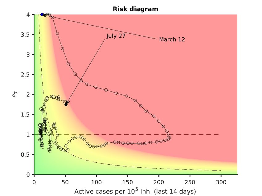
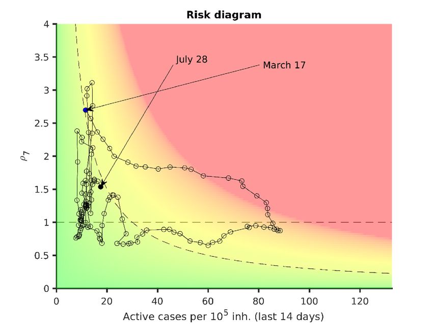
Situation and highlights
The risk diagram has proven to be a very
useful tool for rapidly visualizing and
assessing the epidemiological status of a
state or region. In the risk diagram we see
very easily if the epidemic is spreading
(ρ7> 1) or if it is in the process of control
(ρ7

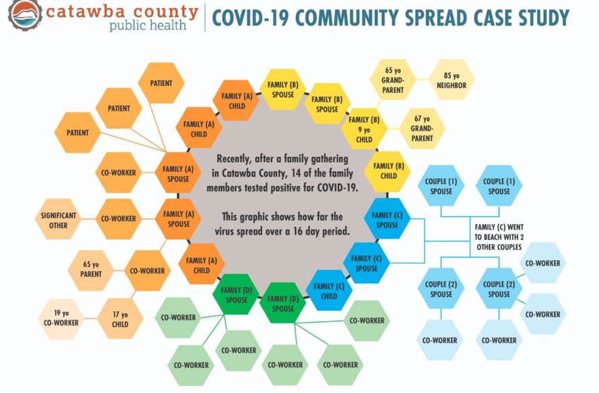
Situation and trends per country
Table of current situation in EU countries. Colour scale is relative except when indicated, this means that it is applied independently to each column, and distinguishes
best (green) form worst (red) situations according to each of the variables. Last column (EPGEST) is assessed with estimated real 14-day attack rate (see report from
22/04 for details). EPGREP is calculated with data reported by countries. EPGREP and EPGEST cannot be compared between them because scales are different, but can
be independently used for estimating risk of countries according to reported or estimated real situation, respectively.

Disclaimer: estimated active cases and estimated 14-day attack rate are assessed by assuming a lethality of 1 % (see report from 20 to 24 April, #37-41). This value can change in
countries where suspicious deaths are reported as well (real values would be lower) and in countries where incidence among elderly people was minor (real values would be higher)
 ρ7 is the average of 7 consecutive ρ, but can still fluctuate. (2,3) EPG stands for Effective Growth Potential. EPGREP is the product of attack-rate of last 14 days per 105 inhabitants by
(1)

ρ7 (empiric reproduction number). EPGEST is the product of estimated real attack-rate of last 14 days per 105 inhabitants and ρ7. Biocom-Cov degree is an epidemiological situation
 4
scale based on the level of last week’s mean daily new cases (https://upcommons.upc.edu/handle/2117/189661, https://upcommons.upc.edu/handle/2117/189808).

Analysis: On the local containment of outbreaks (II). The false sense of security in
exteriors and the focus on voice level.
We have been reporting on the evolution of the outbreak of covid19 that started last month in the city of
Lleida, 200 km west of Barcelona (Figure 1). Since then, Barcelona and its surrounding area has also observed
a large outbreak (Figure 1) which has been growing with empirical reproductive number higher than 2 for
two weeks, with community transmission. In both cases, the transmission is slowing down this week as a
result of the control measures taken by the regional government. Nevertheless, the new outbreak has
stressed the ability of primary care to deal with all cases. We use this assessment to address one of the
drivers of the outbreak in Catalonia, the false sense of security that large gatherings outdoors are riskless.

 Figure 1: Daily new cases in Barcelona and Lleida cities, smoothed with a 7-day
 moving average.

There has been a consistent message that the interiors were dangerous in terms of contagiousness, implicitly
stating that exteriors had less risk, with no mention of voice levels. This could have been read by the
population that outdoors activities are basically safe. The fact is that, as a consequence, Spain has had
multiple activities allowed outdoors. Terraces in bars and restaurants opened very early, like in Spain,
much earlier than cinemas or other indoors activities. The consequences have been dramatic in Catalonia.
A very significant number of clusters has been generated outdoors. As it has been explained by WHO, but
maybe not sufficiently emphasized, the key driver of the outbreaks is the number of drops with infected
quanta. The higher the level of voice, the higher the chances of infection. Indoors can help this driver of
contagion if there is bad ventilation or lack of proper AC filters, but close gatherings outdoors can be, in
principle, as dangerous as indoors. Catalonia is a perfect proof of this concept.
The origin of the confusion comes from the analysis done in Japan regarding outdoor vs indoor activity
https://www.medrxiv.org/content/10.1101/2020.02.28.20029272v2. In the report, the probability of having
infection indoors was reported to be roughly 20 times higher than outdoors. This kind of numbers seem to
suggest that outdoors is save. There is, however, a danger in generalization of different contact networks
and structures. If the main driver of infections is the level of voice and droplets, the use of voice in outdoor
settings can have very important effects on these numbers. To guarantee that the results in Japan can be
generalized to Catalonia, for example, we should guarantee that the average voice level in Japan outdoors is
the same that in Catalonia or, more generally, in Southern Europe. We have looked for bibliography regarding
the typical voice level (in dB) outdoors in Spain vs Japan. There are multiple anthropological reports regarding
the use of voice and the value of silence across different cultures (see for example
https://web.uri.edu/iaics/files/08-Robert-N.-St.-Clair.pdf). The different value of silence has been clearly
documented. Regarding dB measurement, Japan presents very high levels of noise reaching 100 dB due to

 5

warning signs, music and intrusive audio sound. In this sense, sales people scream systematically in the
streets with megaphones. Actually, Spain and Japan cities are systematically on the top of noisiest cities, year
after year 2.
The key problem is that general noise is not relevant, but the use of voice in public gatherings. If we go out
of the core of the cities, into the suburbs, compulsory levels of 45 dB are common in Japan (lower than in a
typical library 3). Even kids playing generate higher levels of noise. This is unheard of in Spain. It is thus clear
that the relation between noise and voice in Catalonia and Japan is very different. It is then not surprising to
observe that the number of clusters in Catalonia outdoors have been pretty significant. We provide here a
list of the most dangerous outdoors environments detected in Catalonia (and also Spain), all of them related
with heavy emissions of droplets.
 • Huge clusters in temporary workers living and working outdoors but sharing those outdoor spaces
 with a large community in Lleida 4. All of these are associated with the fruit pick-up season. It is
 difficult to know the ratio of those infected that lived in community areas indoors vs those living in
 the streets. All of them, however, did work outdoors. Infections in outdoor activity can be very
 important. The physical exercise is large, and distances between workers are not necessarily large.
 • Clusters in parties at the beach. According to the news report 5:
 “Doctors from the Vilassar de Dalt (Maresme) ambulatory yesterday carried out PCR tests on a dozen
 young people with symptoms of fever and diarrhea after having participated a few days ago in a
 massive party on the Palomares beach in Vilassar de Mar… Case zero is a young man from Vilassar
 de Dalt who went to the Primary Care Center yesterday with symptoms of Covid-19. After the tests, it
 was positive, so Salut started all the tracking protocols… Subsequently, a dozen young people also
 showed symptoms of fever and diarrhea after having participated a few days ago in the party.”
 • Clusters in family gatherings and meeting in terraces and outdoor activity. According to health
 authorities in Spain, 40% of the chain infections involving 3 or more people are related with family
 gatherings 6. Detailed figures regarding where those gathering happened are not available. News
 report indicate that outdoor terraces have been present, and that barbecue-like gatherings are main
 drivers. In Spain, these gatherings are mainly outdoors (parks, terraces...). This is very reminiscent of
 large clusters in family barbecues gatherings in the US. Given that we do not have data from Spain,
 we can use data from other similar clusters. More specifically, the next image shows the structure of
 a cluster related with barbecue-gathering in North Carolina (Figure 2). We cannot be sure that the
 barbecue was all outdoor. It can be partially outdoor, and partially indoor. But more importantly,
 some of the members infected others in a beach gathering.

2
 https://www.thelocal.es/20190423/which-cities-in-spain-are-the-noisiest-clue-not-madrid
3
 https://www.ft.com/content/8911cf0a-c3d2-11e4-a02e-00144feab7de
4
 https://www.elperiodico.com/es/sociedad/20200705/rebrote-coronavirus-lleida-confinamiento-crisis-sociales-8027774
5
 https://www.lavanguardia.com/local/maresme/20200710/482203786307/brote-coronavirus-playa-vilassar-de-mar-cabrils-
vilassar-de-dalt-masnou-alella.html
6
 https://elpais.com/sociedad/2020-07-10/el-mapa-de-los-brotes-de-coronavirus-el-40-tiene-su-origen-en-encuentros-
familiares.html

 6

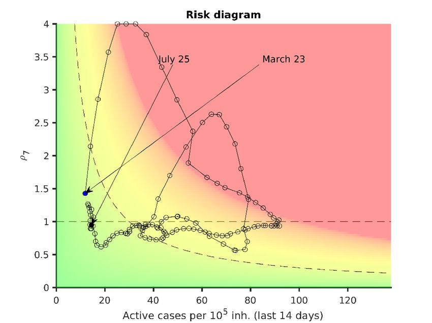
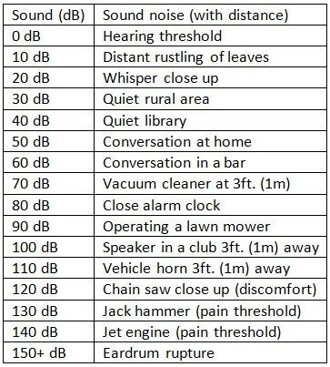
Figure 2: Structure of a cluster related with a barbecue and a beach gathering in
 North Carolina (source: catawbacountync.gov).
In other words, this type of cluster has been typical of Catalonia 7. The number of infections produced
outdoors is large. The gatherings outdoors reverberate into indoors clusters with close contacts at work.

 • Cluster in so-called botellón parties. Botellón parties are outdoor gatherings in the street where,
 generally, young people join economic resources to buy and share bottles of alcohol. Buying full
 bottles are, as a matter of fact, way cheaper than any drink in bar or disco when the content of the
 bottle is split. The image of young people sharing the drinks is common in Spanish streets 8. Clusters
 in these types of gatherings have been reported in all major news outlets.
A very final note is warranted. During the last month, cinemas
and theaters have been open. They had to follow the guidelines
regarding masks and distance. Obviously the level of voice in
the cinemas is very low, basically around 30 dB compared with
a normal conversation of 60 dB (Figure 3). We must remember
here that the decibel scale is not linear but logarithmic. From
30 to 60 dB the intensity of the sound does not double but is
multiplied by 1000. It is thus no surprising that not a single
case of a cluster in cinemas has been reported in Spain.
Actually, we have not been able to identify any cluster in an
indoor cinema anywhere in the world. On the other hand,
clusters of gatherings in the beach or street parties are very
common. In other words, there is no doubt now that an
outdoor family gathering, not to mention a party in the beach, Figure 3: Typical dB scale and sources of that
is, at least, a hundred times more dangerous and riskier than a noise’s level (source:
 https://www.quora.com/How-loud-is-65-
movie-watch gathering in silence. For all we know, given the
zero number of clusters in cinemas, risk in indoors silence gatherings could be thousand or ten-thousand

7
 https://www.lavanguardia.com/vida/20200626/481959375408/brote-coronavirus-vall-aran-barbacoa-amigos.html
8See for example pictures in https://www.burgosconecta.es/sociedad/macrobotellon-wuhan-manchega-20200601130030-
ntrc.html#vca=modulos&vso=burgosconecta&vmc=noticias-rel-1-
cmp&vli=salud&ref=https://www.burgosconecta.es/sociedad/salud/simon-sobre-botellones-20200601182024-ntrc.html or
https://www.laprovincia.es/las-palmas/2020/07/03/botellon-ilegal-vegueta/1297112.html

 7

times lower that most outdoors activities with normal 60 dB-talk interactions. The same can be said about
gathering where people sing. Large clusters in chorus gatherings have become famous 9.
According to https://www.engineeringtoolbox.com/voice-level-d_938.html, in social settings people often
talk with normal voice levels at distances ranging 1 to 4 meters. In outdoor play and recreational areas people
often communicate with raised or very loud voices. Next table shows an estimation of the voice level at
different distances and contexts.
 Table 1: Voice level at different distances and situations (adapted
 from: https://www.engineeringtoolbox.com/voice-level-d_938.html)
 Distance Voice Level (dB)
 Social settings Outdoor play and recreational areas
 (m) Normal Raised Very loud Shouting
 0.3 70 76 82 88
 0.9 60 66 72 78
 1.8 54 60 66 72

It should be clear that we are not saying that indoor activities are not problematic. Close contact at work has
been the focus of major clusters. Similarly, large indoor parties in disco-bars have also been the source of
very large clusters of cases in Spain. There is no doubt that bad ventilation indoors can help infections. But
the same type of large infections is possible outdoors if the same type of party-like behavior is present. What
we are saying is that the focus of health authorities should move from indoor vs outdoor messages into
low versus high voice use. The core problem is not indoor gathering. The core problem is high dB voice use
because of loud conversation.

9
 https://www.cdc.gov/mmwr/volumes/69/wr/mm6919e6.htm

 8

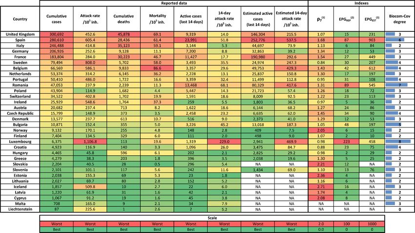
Situation and trends in other countries
Table of current situation in a sample of non-EU countries. Colour scale is relative except when indicated, this means that it is applied independently to each column,
and distinguishes best (green) form worst (red) situations according to each of the variables. EPGREP and EPGEST cannot be compared between them because scales
are different, but can be independently used for estimating risk of countries according to reported or estimated real situation, respectively.

Disclaimer: estimated active cases and estimated 14-day attack rate are assessed by assuming a lethality of 1 % (see report from 20 to 24 April, #37-41). This value can change in
countries where suspicious deaths are reported as well (real values would be lower) and in countries where incidence among elderly people was minor (real values would be higher).

 ρ7 is the average of 7 consecutive ρ, but can still fluctuate. (2,3) EPG stands for Effective Growth Potential. EPGREP is the product of attack-rate of last 14 days per 105 inhabitants by
(1)

ρ7 (empiric reproduction number). EPGEST is the product of estimated real attack-rate of last 14 days per 105 inhabitants and ρ7. Biocom-Cov degree is an epidemiological situation
 9
scale based on the level of last week’s mean daily new cases (https://upcommons.upc.edu/handle/2117/189661, https://upcommons.upc.edu/handle/2117/189808).

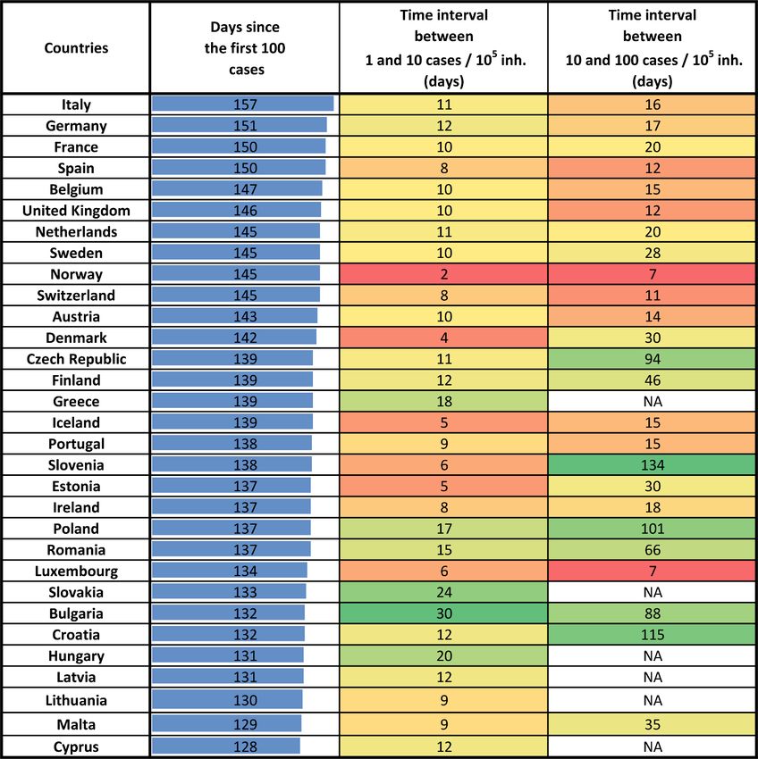
Time indicators by country
These tables summarize a few time indicators for each country: time since 50 cases were reported, time
interval between an attack rate of 1/105 inhabitants and an attack rate of 10/105 inhabitants, and time
interval between attack rates of 10 to 100 per 105 inhabitants (only for countries that have overtaken this
threshold). Data from 2nd July.
EU+EFTA+UK countries

 10

Other countries

 11

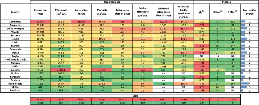
Situation and trends in Italian and Spanish regions
Italy
Data from 29th July

Spain
Data not updated

Disclaimer: estimated active cases and estimated 14-day attack rate are assessed by assuming a lethality of 1 % (see
report from 20 to 24 April, #37-41). This value can change in countries where suspicious deaths are reported as well
(real values would be lower) and in countries where incidence among elderly people was minor (real values would be
higher).
(1)
 ρ7 is the average of 7 consecutive ρ, but can still fluctuate. (2,3) EPG stands for Effective Growth Potential. EPGREP is the
product of attack-rate of last 14 days per 105 inhabitants by ρ7 (empiric reproduction number). EPGEST is the product of
estimated real attack-rate of last 14 days per 105 inhabitants and ρ7. Biocom-Cov degree is an epidemiological situation
scale based on the level of last week’s mean daily new cases (https://upcommons.upc.edu/handle/2117/189661,
https://upcommons.upc.edu/handle/2117/189808).

Long-term predictions are not shown any more, since all Italian and Spanish regions are already in the tail
(see Analysis section in Report #87, https://upcommons.upc.edu/handle/2117/190497).

 12

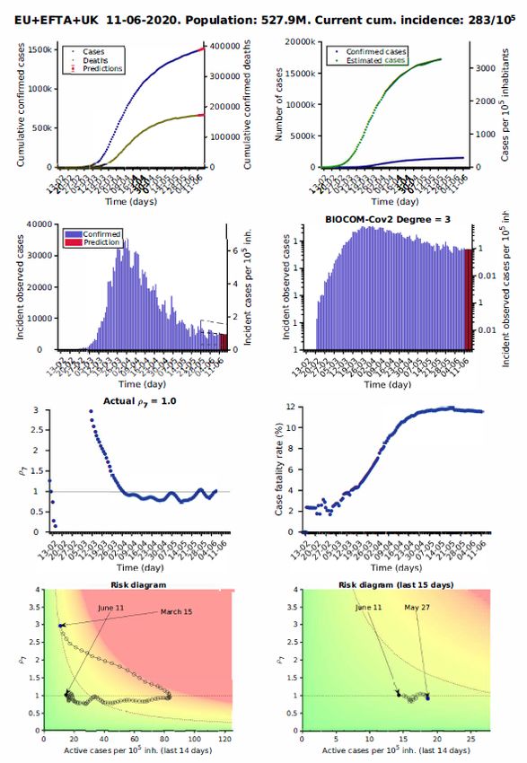
Legend: Countries’ reports details

 Reported
cumulative cases Estimated and
(blue) and deaths reported cases.
 (brown),
 together with
 predictions (red

 Incident Incident observed
observed cases cases in a
 and logarithmic scale,
 predictions. with Biocom-Cov
 degree.

 Evolution of
 empiric
 Case fatality
 reproductive
 rate
 number ρ7

 Risk Risk diagram of
 diagram last 15 days

 13

(1) Analysis and prediction of COVID-19
 for EU+EFTA+UK

Data obtained from https://www.ecdc.europa.eu/en/geographical-distribution-2019-ncov-cases

 14

15

16

17

18

19

20

21

22

23

24

25

26

27

28

29

30

31

32

33

34

35

36

37

38

39

40

41

42

43

44

45

46

(2) Analysis and prediction of COVID-19
 for other countries

Data obtained from https://www.ecdc.europa.eu/en/geographical-distribution-2019-ncov-cases

 47

48

49

50

51

52

53

54

55

56

57

58

59

60

61

62

63

64

65

66

67

68

69

70

71

Methods

 72

Methods
(1) Data source
Data are daily obtained from World Health Organization (WHO) surveillance reports 10, from European Centre
for Disease Prevention and Control (ECDC) 11 and from Ministerio de Sanidad 12. These reports are converted
into text files that can be processed for subsequent analysis. Daily data comprise, among others: total
confirmed cases, total confirmed new cases, total deaths, total new deaths. It must be considered that the
report is always providing data from previous day. In the document we use the date at which the datapoint
is assumed to belong, i.e., report from 15/03/2020 is giving data from 14/03/2020, the latter being used in
the subsequent analysis.

(2) Data processing and plotting
Data are initially processed with Matlab in order to update timeseries, i.e., last datapoints are added to
historical sequences. These timeseries are plotted for EU individual countries and for the UE as a whole:

  Number of cumulated confirmed cases, in blue dots
  Number of reported new cases
  Number of cumulated deaths

Then, two indicators are calculated and plotted, too:

  Number of cumulated deaths divided by the number of cumulated confirmed cases, and reported as
 a percentage; it is an indirect indicator of the diagnostic level.
  ρ: this variable is related with the reproduction number, i.e., with the number of new infections
 caused by a single case. It is evaluated as follows for the day before last report (t-1):
 ( ) + ( − 1) + ( − 2)
 ( − 1) =
 ( − 5) + ( − 6) + ( − 7)
 where Nnew(t) is the number of new confirmed cases at day t.

(3) Classification of countries according to their status in the epidemic cycle
The evolution of confirmed cases shows a biphasic behaviour:

 (I) an initial period where most of the cases are imported;
 (II) a subsequent period where most of new cases occur because of local transmission.

Once in the stage II, mathematical models can be used to track evolutions and predict tendencies. Focusing
on countries that are on stage II, we classify them in three groups:

 • Group A: countries that have reported more than 100 cumulated cases for 10 consecutive days or
 more;
 • Group B: countries that have reported more than 100 cumulated cases for 7 to 9 consecutive days;
 • Group C: countries that have reported more than 100 cumulated cases for 4 to 6 days.

10
 https://www.who.int/emergencies/diseases/novel-coronavirus-2019/situation-reports
11
 https://www.ecdc.europa.eu/en/geographical-distribution-2019-ncov-cases
12
 https://www.mscbs.gob.es/profesionales/saludPublica/ccayes/alertasActual/nCov-China/situacionActual.htm
https://github.com/datadista/datasets/tree/master/COVID%2019 , https://covid19.isciii.es/

 73

(4) Fitting a mathematical model to data

Previous studies have shown that Gompertz model 13 correctly describes the Covid-19 epidemic in all analysed
countries. It is an empirical model that starts with an exponential growth but that gradually decreases its
specific growth rate. Therefore, it is adequate for describing an epidemic that is characterized by an initial
exponential growth but a progressive decrease in spreading velocity provided that appropriate control
measures are applied.

Gompertz model is described by the equation:
 
 − � �· − ·( − 0)
 ( ) = 0

where N(t) is the cumulated number of confirmed cases at t (in days), and N0 is the number of cumulated
cases the day at day t0. The model has two parameters:

  a is the velocity at which specific spreading rate is slowing down;
  K is the expected final number of cumulated cases at the end of the epidemic.

This model is fitted to reported cumulated cases of the UE and of countries in stage II that accomplish two
criteria: 4 or more consecutive days with more than 100 cumulated cases, and at least one datapoint over
200 cases. Day t0 is chosen as that one at which N(t) overpasses 100 cases. If more than 15 datapoints that
accomplish the stated criteria are available, only the last 15 points are used. The fitting is done using Matlab’s
Curve Fitting package with Nonlinear Least Squares method, which also provides confidence intervals of
fitted parameters (a and K) and the R2 of the fitting. At the initial stages the dynamics is exponential and K
cannot be correctly evaluated. In fact, at this stage the most relevant parameter is a. Fitted curves are
incorporated to plots of cumulative reported cases with a dashed line. Once a new fitting is done, two plots
are added to the country report:

  Evolution of fitted a with its error bars, i.e., values obtained on the fitting each day that the analysis
 has been carried out;
  Evolution of fitted K with its error bars, i.e., values obtained on the fitting each day that the analysis
 has been carried out; if lower error bar indicates a value that is lower than current number of cases,
 the error bar is truncated.

These plots illustrate the increase in fittings’ confidence, as fitted values progressively stabilize around a
certain value and error bars get smaller when the number of datapoints increases. In fact, in the case of
countries, they are discarded and set as “Not enough data” if a>0.2 day-1, if K>106 or if the error in K
overpasses 106.

It is worth to mention that the simplicity of this model and the lack of previous assumptions about the Covid-
19 behaviour make it appropriate for universal use, i.e., it can be fitted to any country independently of its
socioeconomic context and control strategy. Then, the model is capable of quantifying the observed
dynamics in an objective and standard manner and predicting short-term tendencies.

(5) Using the model for predicting short-term tendencies
The model is finally used for a short-term prediction of the evolution of the cumulated number of cases. The
predictions increase their reliability with the number of datapoints used in the fitting. Therefore, we consider
three levels of prediction, depending on the country:

13
 Madden LV. Quantification of disease progression. Protection Ecology 1980; 2: 159-176.

 74

• Group A: prediction of expected cumulated cases for the following 3-5 days 14;
 • Group B: prediction of expected cumulated cases for the following 2 days;
 • Group C: prediction of expected cumulated cases for the following day.

The confidence interval of predictions is assessed with the Matlab function predint, with a 99% confidence
level. These predictions are shown in the plots as red dots with corresponding error bars, and also gathered
in the attached table. For series longer than 9 timepoints, last 3 points are weighted in the fitting so that
changes in tendencies are well captured by the model.

(6) Estimating non-diagnosed cases
Lethality of Covid-19 has been estimated at around 1 % for Republic of Korea and the Diamond Princess
cruise. Besides, median duration of viral shedding after Covid-19 onset has been estimated at 18.5 days for
non-survivors 15 in a retrospective study in Wuhan. These data allow for an estimation of total number of
cases, considering that the number of deaths at certain moment should be about 1 % of total cases 18.5 days
before. This is valid for estimating cases of countries at stage II, since in stage I the deaths would be mostly
due to the incidence at the country from which they were imported. We establish a threshold of 50 reported
cases before starting this estimation.

Reported deaths are passed through a moving average filter of 5 points in order to smooth tendencies. Then,
the corresponding number of cases is found assuming the 1 % lethality. Finally, these cases are distributed
between 18 and 19 days before each one.

14
 At this moment we are testing predictions at 4 days for countries with more than 100 cumulated cases for 13-15
consecutive days, and 5 days for 16 or more days.
15
 Zhou et al., 2020. Clinical course and risk factors for mortality of adult
inpatients with COVID-19 in Wuhan, China: a retrospective
cohort study. The Lancet; March 9, doi: 10.1016/S0140-6736(20)30566-3

 75