Understanding and Predicting Importance in Images
←
→
Page content transcription
If your browser does not render page correctly, please read the page content below

Understanding and Predicting Importance in Images

                             Alexander C. Berg1 , Tamara L. Berg1 , Hal Daumé III4 ,
                         Jesse Dodge 6 , Amit Goyal 4 , Xufeng Han1 , Alyssa Mensch 5 ,
                       Margaret Mitchell2 , Aneesh Sood1 , Karl Stratos 3 , Kota Yamaguchi1
                 Stony Brook University 2 University of Aberdeen 3 Columbia University
                   1
      4
        University of Maryland 5 Massachusetts Institute of Technology 6 University of Washington

                         Abstract

   What do people care about in an image? To drive com-
putational visual recognition toward more human-centric
outputs, we need a better understanding of how people per-
ceive and judge the importance of content in images. In
this paper, we explore how a number of factors relate to hu-
man perception of importance. Proposed factors fall into
3 broad types: 1) factors related to composition, e.g. size,
location, 2) factors related to semantics, e.g. category of ob-
ject or scene, and 3) contextual factors related to the likeli-
hood of attribute-object, or object-scene pairs. We explore
these factors using what people describe as a proxy for im-
portance. Finally, we build models to predict what will be
described about an image given either known image con-                   !"#$%&#'()*#+#%,-.)/#%0,#)'1#2*(.,$30#(0#%#$(43$56#
                                                                         !71-$#8318.3#(0#%#2%013#8%,,.(09#(0#%#$(43$#.(03,#'()*#2.(:/56##
tent, or image content estimated automatically by recogni-
                                                                         !;343$%.#8318.3#(0#%#2%013#(0#)*3#$(43$56#
tion systems.
                                                                       Figure 1. An image from the UIUC Pascal sentence dataset [20]
                                                                       with 3 descriptions written by people.

1. Introduction
    Consider Figure 1. Despite the relatively small image              to adopt human-centric views of recognition, especially in
space occupied by the people in the boat, when humans de-              user applications such as image or video search. For exam-
scribe the scene they mention both the people (“3 adults and           ple, in response to an image search for “tree”, returning an
two children”, “Four people”, “Several people”), and the               image with a tree that no person would ever mention is not
boat (“raft”, “canoe”, “canoe”). The giant wooden struc-               desirable.
ture in the foreground is all but ignored, and the cliffs in the          In this paper we consider the problem of understanding
background are only mentioned by one person. This sug-                 and predicting perceived importance of image content. A
gests a significant and interesting bias in perceived content          central question we pose is: what factors do people inher-
importance by human viewers!                                           ently use to determine importance? We address this ques-
    Now that visual recognition algorithms are starting to             tion using descriptions written by people as indicators of
work – we can reliably recognize tens or hundreds of ob-               importance. For example, consider Fig. 2. Despite con-
ject categories [11, 6, 24, 10], and are even beginning to             taining upwards of 20 different objects, people asked to
consider recognition at a human scale [2, 17] – we need                describe the image tend to mention quite similar content
to start looking closely at other questions related to image           aspects: the man, the baby, the beard, and the sling (and
understanding. Current systems would treat recognition of              sometimes the kitchen). This suggests there are some un-
all objects in pictures like Fig. 1 as equally important, de-          derlying consistent factors influencing people’s perception
spite indications that humans do not do so. Because people             of importance in pictures.
are often the end consumers of imagery, we need to be able                We study a number of possible factors related to per-

                                                                   1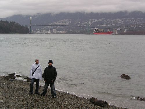
!"#$;+%.2%$".+%.1#4)0%                                                          !"#$%&'%()'(*)%&)+,-./)0%
       1#2%         ,"#.-%                                                        67%#$%&'$'!(%)!+$#2&+%8".*)%"'*&.24%#%*(%++!,-.+'!.2%#%
       /#/3%        /'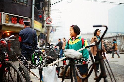
man perspective, including the shift away from purely ob-       factors at scale. However, some factors are still difficult to
ject based outputs, toward including attributes [26, 1, 7],     measure well – e.g. scene, or contextual factors – because
scenes [18, 21], or spatial relationships [15, 13]. Other re-   they require collecting additional content labels not present
lated work includes attempts to compose natural language        in the dataset, somewhat difficult for the large scale Image-
descriptions for images [15, 16, 19, 8]. Especially relevant    CLEF data.
– in fact almost the “dual” to this paper – is recent work          Therefore, we use the UIUC Pascal Sentence data set
in natural language processing predicting whether pieces of     (UIUC), which consists of 1K images subsampled from the
text refer to visual content in an image [3]. However, none     Pascal Challenge [6] with 5 descriptions written by humans
of these approaches focus on predicting perceived impor-        for each image. As with all Pascal images, they are also an-
tance and how it could influence what to recognize in (or       notated with bounding box localizations for 20 object cate-
describe about) an image.                                       gories. This dataset is smaller than the ImageCLEF dataset,
                                                                and is a reasonable size to allow collecting additional la-
1.2. Overview of the Approach                                   bels with Mechanical Turk (Sec 2.2). Crucially this dataset
   We start by describing the data we use for investigating     has also been explored by the vision community, resulting
importance (Sec 2.1), how we gather labels of image con-        in object detectors [10], attribute classifiers [15], and scene
tent (Sec 2.2), and how we map from content to descrip-         classifiers [28] for effectively estimating image content.
tions (Sec 2.3). Next we examine the influence of each of
our proposed importance factors, including compositional        2.2. Collecting Content Labels
(Sec 3.1), semantic (Sec 3.2), and contextual (Sec 3.3). Fi-        We use three kinds of content labels: object labels, scene
nally, we train and evaluate models to predict importance       labels, and attribute labels. Object labels are already present
given known image content (Sec 4.1) or given image con-         in each of our data collections. ImageCLEF images are seg-
tent estimated by computer vision (Sec 4.2).                    mented and each segment is associated with an object cat-
                                                                egory label. In the UIUC dataset there are bounding boxes
2. Data, Content Labels, & Descriptions                         around all instances of the 20 PASCAL VOC objects. To
   To study importance in images we need three things:          gather additional content labels – for scenes and attributes
large datasets consisting of images, ground truth content       in the UIUC dataset – we use Mechanical Turk (MTurk).
in those images, and indicators of perceptually important           To procure scene labels for images, we design a MTurk
content. For the first requirement, we use two large exist-     task that presents an image to a user and asks them to select
ing image collections (described in Sec 2.1). For the sec-      the scene which best describes the image from a list of 12
ond requirement, we use existing content labels or collect      scenes that cover the UIUC images well. Users can also
additional labels using Amazon’s Mechanical Turk service        provide a new scene label through a text box denoted with
(Sec 2.2). For the last requirement, we make use of exist-      “other,” or can select “no scene observed” if they cannot
ing descriptions of the images written by humans. As il-        determine the scene type. In addition, we ask the users to
lustrated in Fig. 2, what people describe when viewing an       rate their categorization, where a rating of 1 suggests that
image can be a useful proxy for perceived importance. Fi-       the scene is only barely interpretable from the image, while
nally, we map between what the humans judge to be impor-        5 indicates that the scene category is obviously depiction.
tant (things mentioned in descriptions) to the labeled image    Each image is viewed and annotated by 5 users.
content by hand or through simple semantic mapping tech-            Our MTurk task for labeling attributes of objects presents
niques (Sec 2.3).                                               the user with a cropped image around each object. Each of
                                                                3430 objects from the UIUC data are presented separately
2.1. Data                                                       to labelers along with a set of possible attributes. Three
   We use two data collections to evaluate our proposed         users select the attributes for each object.
factors for importance: the ImageCLEF dataset [12], and
the UIUC Pascal Sentence dataset [20]. ImageCLEF is a           2.3. Mapping Content Labels to Descriptions
collection of 20K images covering various aspects of con-           We also require a mapping between labeled image con-
temporary life, such as sports, cities, animals, people, and    tent and text descriptions for each image. For example, if
landscapes. The original IAPR TC-12 Benchmark [12] in-          an image contains 2 people as in Fig. 2, we need to know
cludes a free-text description for each image. Crucially,       that the “man” mentioned in description 1 refers to one of
in its expansion (SAIAPR TC-12), each image is also seg-        those people, and the “child” refers to the other person. We
mented into constituent objects and labeled according to a      also need mappings between scene category labels and spe-
set of (275) labels [5]. From here on we will refer to this     cific words in the description, as well as between attribute
dataset, and its descriptions as ImageCLEF. This dataset is     categories and words (e.g. the “bearded man” refers to a
quite large, and allows us to explore some of our proposed      person with a “has beard” attribute). In the case of a small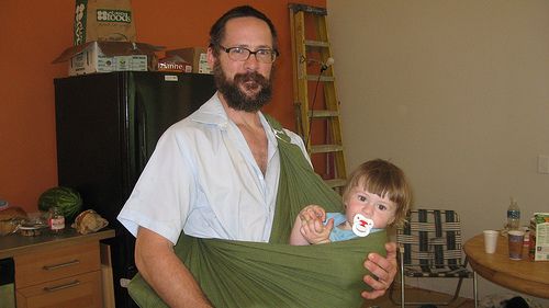
!"#$"%&'"()*+,)-."/%0+                                85#)('-+,)-."/%0+                                                                                                                      !"(.5J.+,)-."/%0+
 8&95+                          >"-)'"(+                      C3D5-.+:B$5+                                                       8-5(5+:B$5+E+F5$&-'"(+8./5(=.4+                                    G(A%A)*+"3D5-.H%-5(5+I)&/+

12+%)&*+3").+"(+.45+   1:;"+#5(+%.)(
Top10       Prob    Last10        Prob                           Rating       1     2       3      4       5
                                                                              Prob      0.15 0.21 0.21 0.22 0.26
             firework 1.00       hand         0.15
             turtle      0.97    cloth        0.15                 Table 5. Probability of Scene term mentioned given Scene depic-
             horse       0.97    paper        0.13                 tion strength (1 implies the scene type is very uncertain, and 5
             pool        0.94    umbrella     0.13                 implies a very obvious example of the scene type, as rated by hu-
             airplane 0.94       grass        0.13                 man evaluators). Scenes are somewhat more likely to be described
             bed         0.92    sidewalk     0.11                 when users provide higher ratings.
             person      0.92    tire         0.11
             whale       0.91    smoke        0.09
             fountain 0.89       instrument 0.07                   ble 3) less semantically salient objects (e.g. chair, potted
             flag        0.88    fabric       0.07                 plant, bottle) are described with lower probability than more
Table 1. Probability of being mentioned when present for various   interesting ones (cow, cat, person, boat).
object categories (ImageCLEF).                                        It is also interesting to note that animate objects are much
                                                                   more likely to be mentioned when present than inanimate
                      Prob-ImageCLEF       Prob-Pascal
                                                                   ones in both datasets (Table 2). From these results one could
                                                                   hypothesize that observers usually perceive (or capture) the
          Animate             0.91             0.84                animate objects as the subject of a photograph and the more
          Inanimate           0.53             0.55                common objects (e.g. sofa, grass, sidewalk) as background
Table 2. Probability of being mentioned when present for Animate   content elements.
versus Inanimate objects.
                                                                   Scene Type & Depiction Strength: In Sec 2.1 we de-
                                                                   scribed our Mechanical Turk experiments to gather scene
           Object       Prob    Object         Prob
                                                                   labels and depiction strength ratings for the UIUC images.
            horse        0.99    bus           0.80                In addition, we also annotate whether the scene category is
            sheep        0.99    motorbike     0.75                mentioned in each image’s associated descriptions. The re-
            train        0.99    bicycle       0.69                lationship between scene type and description is shown in
            cat          0.98    sofa          0.59
                                                                   Table 4. Some scene categories are much more likely to
            dog          0.96    dining table 0.56
                                                                   be described when depicted (e.g. office, kitchen, restaurant)
            aeroplane 0.97       tv/monitor    0.54
            cow          0.95    car           0.43                than others (e.g. river, living room, forest, mountain). In
            bird         0.93    potted plant 0.26                 general we find that the scene category is much more likely
            boat         0.90    bottle        0.26                to be mentioned for indoor scenes (ave 0.25) than for out-
            person       0.81    chair         0.26                door scenes (ave 0.12).
Table 3. Probability of being mentioned when present for various       Finally, we also look at the relationship between scene
object categories (UIUC).                                          depiction strength – whether the scene is strongly obvious
                                                                   to a viewer as rated by human observers – and description.
                                                                   We expect that the more obvious the scene type (e.g. the
categories are more important to human observers than oth-         iconic kitchen depiction in Fig. 3), the more likely it is to
ers. For example, being human we expect that “people” in           be described by a person (e.g. “kitchen in house”). Using
an image will attract the viewers attention and thus will be       a scene word can be more succinct and informative than
more likely to be described. For example, in Fig. 3, 3rd pic-      naming all of the objects in the scene, but the scene type
ture, the caption reads “Girl in the street” despite the large     needs to be relatively obvious for an observer to name it.
and occluding bicycle in front of her.                             We observe (Table 5) that scene depiction strength has some
   Table 1 and Table 3 show the 10 most probable object            correlation with description probability.
types and 10 least probable object types from the Image-
CLEF and UIUC datasets respectively, sorted according to           3.3. Context Factors
the probability of being described when present in an image.           We examine two kinds of contextual factors and their
A few observations can be drawn from these statistics. Very        influence on description. The first is object-scene context,
unusual objects tend to be mentioned; we don’t see fire-           hypothesizing that the setting in which an object is depicted
works very often, so when an image contains one it is likely       will have an impact on whether or not the object will be
to be described. The person category also ranks highly in          described. We visualize the probability of an object being
both lists because of our inherent human tendency to pay           described given that it occurs in a particular scene in Fig. 5.
attention to people. In contrast, the objects deemed non-          Some interesting observations can be made from this plot.
salient tend to be very common ones (sidewalk, tire), too          For example, bicycles in the dining room are more likely to
generic (smoke, cloth), or part of something more salient          be described than those on the street (perhaps because they
(hand). In the UIUC data (Table 3) we observe that (Ta-            are in an unusual setting). Similarly, a TV in a restaurant is
office airport kitchen dining room field living room street river restaurant sky forest mountain
0.29 0.13 0.36 0.21 0.16 0.13 0.18 0.1 0.28 0.18 0.0 0.07
Table 4. Probability of description for each Scene Type.
t
e
offic airp
ort itchen ining eld
k d fi livin
g
stre
et
rive
r
resta
uran y
sk fore
st
mou
ntainant tell
c Model Features Accuracy% (std)
person
car
Baseline (ImageCLEF) 57.5 (0.2)
bus Log Reg (ImageCLEF) Kos + Kol 60.0 (0.1)
table
chair Log Reg (ImageCLEF) Koc 68.0 (0.1)
aeroplane Log Reg (ImageCLEF) Koc +Kos +Kol 69.2 (1.4)
potted plant
bicycle Baseline (UIUC-Kn) 69.7 (1.3)
cat
dog Log Reg (UIUC-Kn) Kos +Kol 69.9 (0.6)
cow Log Reg (UIUC-Kn) Koc 79.8 (1.4)
bottle
train Log Reg (UIUC-Kn) Koc +Kos +Kol 82.0 (0.9)
Baseline (UIUC-Est) 76.5 (1.0)
sheep
tv monitor
sofa Log Reg (UIUC-Est) Eos +Eol 76.9 (1.1)
bird
horse Log Reg (UIUC-Est) Eoc 78.9 (1.4)
motorbike Log Reg (UIUC-Est) Eoc +Eos +Eol 79.52 (1.2)
boat
Table 6. Accuracy of models for predicting whether a given ob-
ject will be mentioned in an image description on the ImageCLEF
and UIUC datasets given known image content (UIUC-Kn) and
Figure 5. The impact of Object-Scene context on description. Col- visual recognition estimated image content (UIUC-Est). Features
ors indicate the probability of an object being mentioned given – Koc for known object category, Kos for known object size, Kol
that it occurs in a particular scene category (red - high, blue - low). from known object location, Eoc estimated object category, Eos es-
Objects in relatively unusual settings (e.g. bicycles in the dining timated object size, Eol estimated object location.
room) are more often described than those in ordinary settings (e.g.
bicycles in the street).
0.6
1
described, followed by beard, wearing glasses, and wear-
%&'(")$ !"#$
0.9
0.5 0.8
0.7
ing shirts (a similar ordering to how usual or unusual these
attributes of people tend to be). For cows, eating is the
0.4
0.6
0.3 0.5
most likely attribute, over actions like standing or sitting
0.4
0.2 0.3
0.2
0.1
0
0.1
0
(lying down). Color attributes also seem to be described
frequently. Similar observations were made for the other
eating
sitting
standing
white
brown
spotted
black
wearHat
wearGlasses
wearShirt
sitting
beard
riding
eating
man
woman
boy
girl
baby
smiling
walking
talk
holding
standing
object categories.
Figure 6. The impact of Attribute-Object context, showing the
probability of an attribute being mentioned given that it occurs 4. Predicting Importance
with a particular object. More unusual attributes (e.g.riding per-
son) tend to be mentioned more often than relatively common at- We train discriminative models to predict importance –
tributes (e.g.standing). using presence or absence in a description as proxy for an
importance label. These models predict importance given as
input: known image content (Sec 4.1), or estimates of im-
more likely to be described than a TV in a living rooms. In age content from visual recognition systems (Sec 4.2). For
images where the scene is unclear (perhaps because they are each input scenario, we train 3 kinds of models: a) models
object focused images), the objects present are very likely to predict whether an object will be mentioned, b) models
to be described. to predict whether a scene type will be mentioned, and c)
The second contextual factor we explore is attribute- models for predicting whether an attribute of an object will
object context. Here we compute the probability of an at- be mentioned. We use four fold cross validation to train
tribute being described given that it occurs as a modifier for and estimate the accuracy of our learned models. This is
a particular object category. Example results for the “per- repeated 10 time with different random splits of the data in
son” and “cow” categories are shown in Fig. 6. Notice that order to estimate the mean and standard deviation of the ac-
for person, riding is more likely to be described than other curacy estimates. Logistic Regression is used for prediction
actions (e.g. sitting, smiling), perhaps because it is a more with regularization trade-off, C, selected by cross-validation
unusual activity. Wearing a hat is also more likely to be on subsets of training data.
Model                    Features    Accuracy% (std)            Results are shown in Table 7. The baseline – always predict-
      Baseline (UIUC-Kn)                      86.0 (0.2)              ing “No” scene mentioned – obtains an accuracy of 86.0%.
      Log Reg (UIUC-Kn)        Ksc +Ksr       96.6 (0.2)              Prediction using image scene type and rating improves this
       Log Reg (UIUC-Est)         Esd         87.4 (1.3)              significantly to 96.6%.
Table 7. Accuracy of models for predicting whether a particular       Attribute Prediction: We train one model for each com-
scene will be mentioned in the UIUC dataset given known (UIUC-        mon attribute category (categories described at least 100
Kn) and visual recognition estimated image content (UIUC-Est).        times in the UIUC dataset). For example, the “pink” model
Features – Ksc indicates known scene category, Ksr user provided      will predict: given an object and its appearance attributes,
scene depiction rating, and Esd estimated scene descriptor (classi-   whether the attribute term “pink” will appear in the descrip-
fication scores for 26 common scene categories).
                                                                      tion associated with the image containing the detection.
                                                                      Positive samples for an attribute model are those detections
      Model                    Features    Accuracy% (std)            where at least one human image description contains the
      Baseline (UIUC-Kn)                      96.3 (.01)              attribute term, negative samples the rest. Our input descrip-
      Log Reg (UIUC-Kn)        Kac + Koc      97.0 (.01)              tor for the model is a binary vector encoding both object
       Log Reg (UIUC-Est)        Ead +Eoc      96.7 (.01)             category and attribute category (to account for attribute se-
Table 8. Accuracy of models for predicting whether a specific         mantics and attribute-object context). Results are shown in
attribute type will be mentioned in the UIUC dataset given            Table 8. The baseline – always predicting “No” attribute
known (UIUC-Kn) and visual recognition estimated image content        mentioned for all detections – obtains an accuracy of 96.3%
(UIUC-Est). Features – Kac known attribute category, Koc known        due to apparent human reluctance to utilize attribute terms.
object category, Eoc estimated object detection category, Ead esti-   Our model improves prediction accuracy to 97.0%.
mated attribute descriptor (vector of predictions from 21 attribute
classifiers on the object detection window).                          4.2. Predicting Importance from Estimated Content
                                                                         Next, we complete the process so that importance can
                                                                      be predicted from images using computer vision based es-
4.1. Predicting Importance from Known Content                         timates of image content. Specifically we start with a) an
Object Prediction: We train a model to predict: given an              input image, then b) estimates of image content are made
object and its localization (bounding box), whether it will           using state of the art visual recognition methods, and finally
be mentioned in descriptions written by human observers.              c) models predict what objects, scenes, and attributes will
We first look at a simple baseline, predicting “Yes” for ev-          be described by a human viewer. Recognition algorithms
ery object instance. This provides reasonably good accu-              estimate 3 kinds of image content on the UIUC dataset: ob-
racy (Table 6), 57.5% for ImageCLEF and 69.7% for UIUC.               jects, attributes, and scenes. Objects for the 20 Pascal cate-
Next we train several models using features based on ob-              gories are detected using Felzenszwalb et al.’s mixtures of
ject size, location, and type – where size and location are           deformable part models [9]. 21 visual attribute classifiers,
each encoded as a number ∈ [0, 1], and type is encoded in             including color, texture, material, or general appearance
a binary vector with a 1 in the kth index indicating the kth          characteristics [15] are used to compute a 21-dimensional
object category (out of 143 categories for ImageCLEF and              appearance descriptor for detected objects. We obtain scene
20 for UIUC). Results are shown in Table 6, with full model           descriptors for each image by computing scores for 26 com-
accuracies (using all features) of 69.2% and 82.0% respec-            mon scene categories using the SUN dataset classifiers [28].
tively on the two datasets. Interestingly, we observe that for        Object Prediction: For objects, we train models similar
both datasets, the semantic object category feature – not in-         to Sec 4.1, except using automatically detected object type,
cluded in some previous studies predicting importance – is            size, and location as input features. Results are shown in
the strongest feature for predicting whether an object will           the last 4 rows of Table 6. Note that though the object de-
be described, while compositional features are less helpful.          tectors are somewhat noisy, we get comparable results to
Scene Prediction: We train one model for each common                  using known ground truth content (and better results than
scene category (categories described at least 50 times). For          the baseline of classifying all detections as positive). This
example, the kitchen model will predict: given an image               may be because the detectors most often miss detections of
and its scene type, whether the term “kitchen” will appear in         small, background, or occluded objects – those that are also
the description associated with that image. Positive samples          less likely to be described. Performance of our complete
for a scene model are those images where at least one hu-             model is 79.5% compared to the baseline of 76.5%.
man description contains that scene category, negative sam-           Scene Prediction: As in Sec 4.1, for each scene category
ples are the rest. Our descriptor is again a binary vector,           we train a model to predict: given an image whether that
this time encoding image scene type, plus an additional in-           scene type will be mentioned in the associated description.
dex corresponding to user provided rating of scene strength.          However, here we use our 26 dimensional scene descriptor
as the feature. Results are shown in Table 7 bottom row. [7] A. Farhadi, I. Endres, D. Hoiem, and D. A. Forsyth. Describ-
Although the set of scenes used to create our descriptor are ing objects by their attributes. In CVPR, 2009. 3
not exactly the same as the set of described scene categories [8] A. Farhadi, M. Hejrati, A. Sadeghi, P. Young, C. Rashtchian,
in the dataset, we are still able to obtain a classification ac- J. Hockenmaier, and D. Forsyth. Every picture tells a story:
curacy of 87.4% compared to the baseline of 86.0%. Generating sentences for images. In ECCV, 2010. 3
[9] P. F. Felzenszwalb, R. B. Girshick, and D. McAllester.
Attribute Prediction: As in Sec 4.1, for each attribute we Discriminatively trained deformable part models, release 4.
train a model to predict: given an object detection, what http://people.cs.uchicago.edu/ pff/latent-release4/. 7
attribute terms will be used in an associated image descrip- [10] P. F. Felzenszwalb, R. B. Girshick, D. Mcallester, and D. Ra-
tion. We use our 21d attribute descriptor as a feature vector. manan. Object detection with discriminatively trained part
Results are shown in Table 8 bottom. Attribute prediction based models. PAMI, 32(9), Sep 2010. 1, 3
based on estimated attribute descriptor and object category [11] G. Griffin, H. AD, and P. P. The caltech-256. In Caltech
yields 96.7% compared to the baseline of 96.3%. Technical Report, 2006. 1
[12] M. Grubinger, P. D. Clough, H. Mller, and T. Deselaers. The
5. Discussion and Conclusion iapr benchmark: A new evaluation resource for visual infor-
mation systems. In LRE, 2006. 3
We have proposed several factors related to human per- [13] A. Gupta and L. S. Davis. Beyond nouns: Exploiting prepo-
ceived importance, including factors related to image com- sitions and comparative adjectives for learning visual classi-
position, semantics, and context. We first explore the fiers. In ECCV, 2008. 3
impact of these factors individually on two large labeled [14] S. J. Hwang and K. Grauman. Accounting for the relative
datasets. Finally, we demonstrate discriminative methods importance of objects in image retrieval. In BMVC, 2010. 2
to predict object, scene and attribute terms in descriptions [15] G. Kulkarni, V. Premraj, S. Dhar, S. Li, Y. Choi, A. C. Berg,
given either known image content, or content estimated by and T. L. Berg. Babytalk: Understanding and generating
state of the art visual recognition methods. Classification simple image descriptions. In CVPR, 2011. 3, 7
[16] S. Li, G. Kulkarni, T. L. Berg, A. C. Berg, and Y. Choi. Com-
given known image content demonstrates significant perfor-
posing simple image descriptions using web-scale n-grams.
mance improvements over baseline predictions. Classifica-
In CoNLL, 2011. 3
tion given noisy computer vision estimates also produces [17] Y. Lin, F. Lv, S. Zhu, M. Yang, T. Cour, K. Yu, L. Cao, and
smaller, but intriguing, improvements over the baseline. T. Huang. Large-scale image classification: Fast feature ex-
Acknowledgments: Support of the 2011 JHU-CLSP Sum- traction and svm training. In CVPR, 2011. 1
mer Workshop Program. T.L.B and K.Y. were supported [18] A. Oliva and A. Torralba. Building the gist of a scene: the
in part by NSF CAREER #1054133; A.C.B. was partially role of global image features in recognition. Visual Percep-
supported by the Stony Brook University Office of the Vice tion, Progress in Brain Research, pages 23–36, 2006. 3
President for Research; H.D.III and A.G. were partially sup- [19] V. Ordonez, G. Kulkarni, and T. L. Berg. Im2text: Describ-
ported by NSF Award IIS-1139909. ing images using 1 million captioned photographs. In NIPS,
2011. 3
[20] C. Rashtchian, P. Young, M. Hodosh, and J. Hockenmaier.
References Collecting image annotations using amazon’s mechanical
[1] T. L. Berg, A. C. Berg, and J. Shih. Automatic attribute dis- turk. In NAACL HLT Workshop, 2010. 1, 3
covery and characterization from noisy web data. In ECCV, [21] B. C. Russell, A. Torralba, K. P. Murphy, and W. T. Freeman.
2010. 3 Labelme: a database and web-based tool for image annota-
[2] J. Deng, A. C. Berg, K. Li, and L. Fei-Fei. What does classi- tion. IJCV, 77:157–173, may 2008. 2, 3
fying more than 10,000 image categories tell us? In ECCV, [22] M. Spain and P. Perona. Some objects are more equal than
2010. 1 others: measuring and predicting importance. In ECCV,
[3] J. Dodge, A. Goyal, X. Han, A. Mensch, M. Mitchell, 2008. 2, 4
K. Stratos, K. Yamaguchi, Y. Choi, H. D. III, A. C. Berg, [23] M. Spain and P. Perona. Measuring and predicting object
and T. L. Berg. Detecting visual text. In NAACL, 2012. 3 importance. IJCV, 2010. 2, 4
[4] L. Elazary and L. Itti. Interesting objects are visually salient. [24] M. Varma and D. Ray. Learning the discriminative power-
Journal of Vision, 8:1–15, March 2008. 2 invariance trade-off. In ICCV, 2007. 1
[5] H. J. Escalante, C. Hernandez, J. Gonzalez, A. Lopez, [25] L. von Ahn and L. Dabbish. Labeling images with a com-
M. Montes, E. Morales, L. E. Sucar, and M. Grubinger. The puter game. In CHI, pages 319–326, 2004. 2
segmented and annotated iapr tc-12 benchmark. In CVIU, [26] G. Wang and D. Forsyth. Joint learning of visual attributes,
2009. 3 object classes and visual saliency. In ICCV, 2009. 3
[6] M. Everingham, L. V. Gool, C. Williams, and A. Zis- [27] Z. Wu and M. Palmer. Verb semantics and lexical selection.
serman. Pascal visual object classes challenge re- In ACL, 1994. 4
sults. Technical report, 2005. unpublished manuscript [28] J. Xiao, J. Hays, K. Ehinger, A. Oliva, and A. Torralba. Sun
circulated on the web, URL is http://www.pascal- database: Large-scale scene recognition from abbey to zoo.
network.org/challenges/VOC/voc/index.html. 1, 3 In CVPR, 2010. 3, 7You can also read