Beyond PASCAL: A Benchmark for 3D Object Detection in the Wild
←
→
Page content transcription
If your browser does not render page correctly, please read the page content below
Beyond PASCAL: A Benchmark for 3D Object Detection in the Wild
Yu Xiang Roozbeh Mottaghi Silvio Savarese
University of Michigan Stanford University Stanford University
yuxiang@umich.edu roozbeh@cs.stanford.edu ssilvio@stanford.edu
Abstract
3D object detection and pose estimation methods have
become popular in recent years since they can handle am-
biguities in 2D images and also provide a richer descrip-
tion for objects compared to 2D object detectors. How-
ever, most of the datasets for 3D recognition are limited to
a small amount of images per category or are captured in
controlled environments. In this paper, we contribute PAS-
CAL3D+ dataset, which is a novel and challenging dataset
for 3D object detection and pose estimation. PASCAL3D+
augments 12 rigid categories of the PASCAL VOC 2012 [4]
with 3D annotations. Furthermore, more images are added
for each category from ImageNet [3]. PASCAL3D+ images
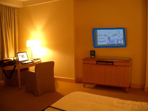
Figure 1. Example of annotations in our dataset. The annotators
exhibit much more variability compared to the existing 3D select a 3D CAD model from a pool of models and align it to the
datasets, and on average there are more than 3,000 object object in the image. Based on the 3D geometry of the model and
instances per category. We believe this dataset will provide the annotated 2D locations of a set of landmarks, we automatically
a rich testbed to study 3D detection and pose estimation compute the azimuth, elevation and distance of the camera (shown
and will help to significantly push forward research in this in blue) with respect to the object. Images are uncalibrated, so the
area. We provide the results of variations of DPM [6] on camera can be at any arbitrary location.
our new dataset for object detection and viewpoint estima-
tion in different scenarios, which can be used as baselines
for the community. Our benchmark is available online at datasets have been introduced [22, 20, 25, 8, 19]. However,
http://cvgl.stanford.edu/projects/pascal3d the current 3D datasets have a number of drawbacks as well.
One drawback is that the background clutter is often lim-
ited and therefore methods trained on these datasets cannot
1. Introduction generalize well to real-world scenarios, where the variabil-
ity in the background is large. Another drawback is that
In the past decade, several datasets have been intro- some of these datasets do not include occluded or truncated
duced for classification, detection and segmentation. These objects, which again limits the generalization power of the
datasets provide different levels of annotation for images relevant learnt models. Moreover, the existing datasets typ-
ranging from object category labels [5, 3] to object bound- ically only provide 3D annotation for a few object classes
ing box [7, 4, 3] to pixel-level annotations [23, 4, 28]. Al- and the number of images or object instances per category is
though these datasets have had a significant impact on ad- usually small, which prevents the recognition systems from
vancing image understanding methods, they have some ma- learning robust models for handling intra-class variations.
jor limitations. In many applications, a bounding box or Finally and most critically, most of these datasets supply
segmentation is not enough to describe an object, and we annotations for a small number of viewpoints. So they are
require a richer description for objects in terms of their 3D not suitable for object detection methods aiming at estimat-
pose. Since these datasets only provide 2D annotations, ing continuous 3D pose, which is a key component in var-
they are not suitable for training or evaluating methods that ious scene understanding or robotics applications. In sum-
reason about 3D pose of objects, occlusion or depth. mary, it is necessary and important to have a challenging 3D
To overcome the limitations of the 2D datasets, 3D benchmark which overcomes the above limitations.
1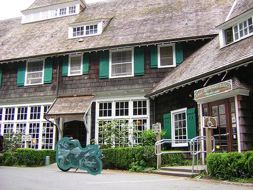
PASCAL3D+ (ours) ETH-80 [13] [26] 3DObject [22] EPFL Car [20] [27] KITTI [8] NYU Depth [24] NYC3DCars [19] IKEA [15]
# of Categories                        12              8      2         10           1        4        2          894             1          11
Avg. # Instances per Category        ∼3000            10     ∼140       10           20      ∼660    80,000       39            3,787        ∼73
Indoor(I) / Outdoor(O)                Both             I     Both      Both           I      Both      O           I              O           I
Cluttered Background                   3              7       3         7            7        3        3           3              3           3
Non-centered Objects                   3              7       3         7            7        7        3           3              3           3
Occlusion Label                        3              7       7         7            7        7        3           3              3           7
Orientation Label                      3              3       3         3            3        3        3           7              3           3
Dense Viewpoint                        3              7       7         7            7        3        3           7              3           3
                                Table 1. Comparison of our PASCAL3D+ dataset with some of the other 3D datasets.

    Our contribution in this work is a new dataset, PAS-                        tics such as viewpoint distribution and variations in degree
CAL3D+. Our goal is to overcome the shortcomings of the                         of occlusion . Section 4 describes the annotation tool and
existing datasets and provide a challenging benchmark for                       the challenges for annotating 3D information in an uncon-
3D object detection and pose estimation. In PASCAL3D+,                          strained setting. Section 5 explains the details of our base-
we augment the 12 rigid categories in the PASCAL VOC                            line experiments, and Section 6 concludes the paper.
2012 dataset [4] with 3D annotations. Specifically, for each
category, we first download a set of CAD models from                            2. Related Work
Google 3D Warehouse [1], which are selected in such a
way that they cover the intra-class variability. Then each                          We review a number of commonly used datasets for 3D
object instance in the category is associated with the closest                  object detection and pose estimation. ETH-80 dataset [13]
CAD model in term of 3D geometry. Besides, several land-                        provides a multi-view dataset of 8 categories (e.g., fruits
marks of these CAD models are identified in 3D, and the                         and animals), where each category contains 10 objects ob-
2D locations of the landmarks are labeled by annotators. Fi-                    served from 41 views, spaced equally over the viewing
nally, using the 3D-2D correspondences of the landmarks,                        hemisphere. The background is almost constant for all of
we compute an accurate continuous 3D pose for each object                       the images, and the objects are centered in the image. [26]
in the dataset. As a result, the annotation of each object con-                 introduces another multi-view dataset that includes motor-
sists of the associated CAD model, 2D landmarks and 3D                          bike and sport shoe categories in more challenging real-
continuous pose. In order to make our dataset large scale,                      world scenarios. There are 179 images and 101 images
we add more images from ImageNet [3] for each category.                         corresponding to each category respectively. On average
In total, more than 20,000 additional images with 3D an-                        a motorbike is imaged from 11 views. For shoes, there are
notations are included. Figure 1 shows some examples in                         about 16 views around each instance taken at 2 different ele-
our dataset. We also provide baseline results for object de-                    vations. 3DObject dataset [22] provides 3D annotations for
tection and pose estimation on our new dataset. The results                     10 everyday object classes such as car, iron, and stapler.
show that there is still a large room for improvement, and                      Each category includes 10 instances observed from differ-
this dataset can serve as a challenging benchmark for future                    ent viewpoints. EPFL Car dataset [20] consists of 2,299
visual recognition systems.                                                     images of 20 car instances at multiple azimuth angles. The
    There are several advantages of our dataset: i) PAS-                        elevation and distance is almost the same for all of these in-
CAL images exhibit a great amount of variability and bet-                       stances. Table-Top-Pose dataset [25] contains 480 images
ter mimic the real-world scenarios. Therefore, our dataset                      of 3 categories (mouse, mug, and stapler), where each con-
is less biased compared to datasets which are collected in                      sists of 10 instances under 16 different poses.
controlled settings (e.g., [22, 20]). ii) Our dataset includes                      These datasets exhibit some major limitations. Firstly,
dense and continuous viewpoint annotations. The existing                        most of them have more or less clean background. There-
3D datasets typically discretize the viewpoint into multi-                      fore, methods trained on them will not be able to han-
ple bins (e.g., [13, 22]). iii) On average, there are more                      dle cluttered background, which is common in real-world
than 3,000 object instances per category. Hence, detectors                      scenarios. Secondly, these datasets only include a limited
trained on our dataset can have more generalization power.                      number of instances, which makes it difficult for recogni-
iv) Our dataset contains occluded and truncated objects,                        tion methods to learn intra-class variations. To overcome
which are usually ignored in the current 3D datasets. v)                        these issues, more challenging datasets have been proposed.
Finally, PASCAL is the main benchmark for 2D object de-                         ICARO [16] contains viewpoint annotations for 26 object
tection. We hope our efforts on providing 3D annotations to                     categories. However, the viewpoints are sparse and not
PASCAL can benchmark 2D and 3D object detection meth-                           densely annotated. [27] provides 3D pose annotations for
ods with a common dataset.                                                      a subset of 4 categories of the ImageNet dataset [3]: bed
    The next section describes the related work and other 3D                    (400 images), chair (770 images), sofa (800 images) and
datasets in the literature. Section 3 provides dataset statis-                  table (670 images). Since the ImageNet dataset is mainly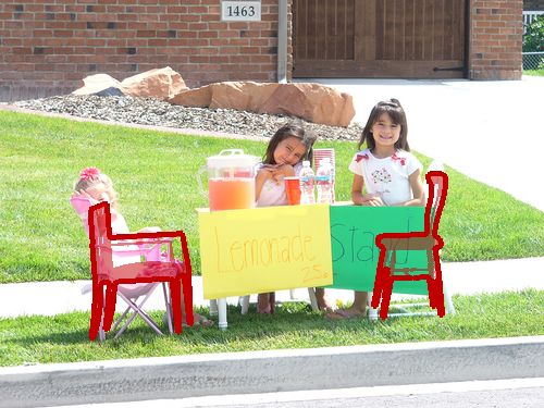
designed for the classification task, the objects in the dataset                        6000

are usually not occluded and they are roughly centered. The                             5000

                                                                       # of instances
KITTI dataset [8] provides 3D labeling for two categories                               4000

(car and pedestrian), where there are 80K instances per                                 3000

category. The images of this dataset are limited to street                              2000

scenes, and all of the images have been obtained by cam-                                1000

eras mounted on top of a car. This may pose some issues                                   0
                                                                                               -85 -75 -65 -55 -45 -35 -25 -15 -5 5 15 25 35 45 55 65 75 85
concerning the ability to generalize to other scene types.                                                              Degrees
More recently, NYC3DCars dataset [19] has been intro-
duced, which contains information such as 3D vehicle an-           Figure 3. Elevation distribution. The distribution of elevation
notations, road segmentation and direction of movement.            among the PASCAL images across all the categories.
Although the imagery is unconstrained for this dataset in
terms of camera type or location, the images are constrained
                                                                   total, there are 13,898 object instances that appear in 8,505
to street scenes of New York. Also, the dataset contains only
                                                                   PASCAL images. Furthermore, we downloaded 22,394 im-
one category. [15] provides dense 3D annotations for some
                                                                   ages from ImageNet [3] for the 12 categories. For the Ima-
of the IKEA objects. Their dataset is also limited to indoor
                                                                   geNet images, the objects are usually centered without oc-
images and the number of instances per category is small.
                                                                   clusion and truncation. On average, there are more than
    Simultaneous use of 2D information and 3D depth makes
                                                                   3,000 instances per category in our PASCAL3D+ dataset.
the recognition systems more powerful. Therefore, various
datasets have been collected by RGB-D sensors (such as                 The annotation of an object contains the azimuth, ele-
Kinect). RGB-D Object Dataset [12] contains 300 physi-             vation and distance of the camera pose in 3D (we explain
cally distinct objects organized into 51 categories. The im-       how the annotation is obtained in the next section). More-
ages are captured in a controlled setting and have a clean         over, we assign a visibility state to landmarks that we iden-
background. Berkeley 3-D Object Dataset [11] provides              tify for each category: 1) visible: the landmark is visible
annotation for 849 images of over 50 classes in real office        in the image. 2) self-occluded: the landmark is not visi-
environments. NYU Depth [24] includes 1,449 densely la-            ble due to the 3D geometry and the pose of the object. 3)
beled pairs of aligned RGB and depth images. The dataset           occluded-by: the landmark is occluded by an external ob-
includes 35,064 distinct instances, which are divided into         ject. 4) truncated: the landmark appears outside the image
894 classes. SUN3D [29] is another dataset of this type,           area. 5) unknown: none of the above four states. To ensure
which provides annotations for scenes and objects. There           high quality labeling, we hired annotators for the annotation
are three limitations for these types of datasets that make        instead of posting the task on crowd-sourcing platforms.
them undesirable for 3D object pose estimation: i) They                Figure 2 shows the distribution of azimuth among the
are limited to indoor scenes as the current common RGB-D           PASCAL images for the 12 categories, where azimuth 0◦
sensors have a limited range. ii) They do not provide the ori-     corresponds to the frontal view of the object. As expected,
entation for objects (they just provide the depth). iii) Their     the distribution of viewpoints is biased. For example, very
average number of images per category is small.                    few images are taken from the back view (azimuth 180◦ )
    Our goal for providing a novel dataset is to eliminate the     of sofa since the back of sofa is usually against a wall. For
mentioned shortcomings of other datasets, and enhance 3D           tvmonitor, there is also a high bias towards the frontal view.
object detection and pose estimation methods by training           Since bottles are usually symmetric, the distribution is dom-
and evaluating them on a challenging and real world bench-         inated by azimuth angles around zero. The distribution of
mark. Table 1 shows a comparison between our dataset and           elevation among the PASCAL images across all categories
some of the most relevant datasets mentioned above.                is shown in Figure 3. It is evident that there is large vari-
                                                                   ability in the elevation as well. These statistics show that
                                                                   our dataset has a fairly good distribution in pose variation.
3. Dataset Details and Statistics
                                                                       We also analyze the object instances based on their de-
   We describe the details of our PASCAL3D+ dataset and            gree of occlusion. The statistics in Figure 4 show that PAS-
provide some statistics. We annotated the 3D pose densely          CAL3D+ is quite challenging as it includes object instances
for all of the object instances in the trainval subset of          with different degrees of occlusion. The main goal of most
PASCAL VOC 2012 detection challenge images (including              previous 3D datasets was to provide a benchmark for ob-
instances labeled as ‘difficult’). We consider the 12 rigid        ject pose estimation. So they usually ignored occluded or
categories of PASCAL VOC, since estimating the pose of             truncated objects. However, handling occlusion and trunca-
the deformable categories is still an open problem. These          tion is important for real world applications. Therefore, a
categories are aeroplane, bicycle, boat, bottle, bus, car,         challenging dataset like ours can be useful. In Figure 4, we
chair, diningtable, motorbike, sofa, train and tvmonitor. In       divide the object instances into three classes based on the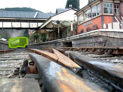
aeroplane bicycle boat bottle bus car
90 100 90 60 90 100 90 1500 90 150 90 250
120 60 120 60 120 60 120 60 120 60
80 80 120 60
40 200
60 60 1000 100
150 30 150 30 150 30 150
40 40 150 30 150 30 150 30
20 500 50 100
20 20
50
180 0 180 0 180 0 180 0 180 0 180 0
210 330 210 330 210 330 210 330 210 330 210 330
240 300 240 300 240 300 240 300 240 300 240 300
270 270 270 270 270 270
chair diningtable motorbike sofa train tvmonitor
90 250 90 250 90 60 90 90 150
200 90 250
120 60 120 60 120 60 120 60 120 60
200 200 120 60
40 150 200
150 150 100
150 30 150 30 150 30 100 150
100 100 150 30 150 30 150 30
20 50 100
50 50 50
50
180 0 180 0 180 0 180 0 180 0 180 0
210 330 210 330 210 330 210 330 210 330 210 330
240 300 240 300 240 300 240 300 240 300 240 300
270 270 270 270 270 270
Figure 2. Azimuth distribution. Polar histograms show the distribution of azimuth among the PASCAL images for each object category.
Aeroplane Bicycle Boat Bottle Bus
5% 4% 3%
7%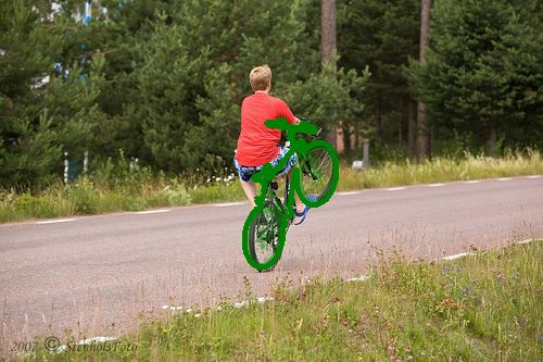
(a) Aeroplane

                                                                 (b) Sofa
Figure 5. Examples of 3D CAD models used for annotation. To better capture intra-class variability of object categories, different types of
CAD models are chosen. The red points represent the identified landmarks.

which are shown with red circles in Figure 5. The land-                 landmarks to obtain the continuous pose of the object:
marks are chosen such that they are shared among instances
                                                                                                    L
in a category and can be identified easily in the images.                                           X
Most of the landmarks correspond to the corners in the                                        min         ||xi − x̃i ||2 ,             (1)
                                                                                              R,t
                                                                                                    i=1
CAD models. The task of annotators is to select the closest
CAD model for an object instance in terms of 3D geome-                  where L is the number of visible landmarks and x̃i is the an-
try and label the landmarks of the CAD model on the 2D                  notated landmark location in the image. By solving the min-
image. Then we use these 2D annotations of the landmarks                imization problem (1), we can find the rotation matrix R and
and their corresponding locations on the 3D CAD models                  the translation vector t, which provide the azimuth, eleva-
to find the azimuth, elevation and distance of the camera               tion and distance of the object pose. This is the well-studied
pose in 3D for each object instance. A visualization of our             Perspective-n-Points (PnP) problem for which various solu-
annotation tool is shown in Figure 6. The annotator first               tions (e.g., [18, 2, 14]) exist. We use the constrained non-
selects the 3D CAD model that best resembles the object                 linear optimization implementation of MATLAB to solve
instance. Then, he/she rotates the 3D CAD model until it                (1). For degenerate cases, where there are not enough land-
is aligned with the object instance visually. The alignment             marks visible to compute the pose (less than 2 landmarks),
provides us with rough azimuth and elevation angles, which              we use the rough azimuth and elevation specified by the an-
are used as initialization in computing the continuous pose.            notator instead.
Based on the 3D geometry and the rough pose of the CAD
model (after alignment), we compute the visibility of the               5. Baseline Experiments
landmarks. After this step, we show the visible (not self-
occluded) landmarks on the 3D CAD model one by one and                     In this section, we provide baseline results in terms of
ask the annotator to mark their corresponding 2D location in            object detection, viewpoint estimation and segmentation.
the image. For occluded or truncated landmarks, the anno-               We also show that how well the baseline method can han-
tator provides its visibility status as explained in Section 3.         dle different degrees of occlusion. For all the experiments
    As the result of the annotation, for each object instance           below, we use the train subset of PASCAL VOC 2012
in the dataset, we obtain the correspondences between 3D                (detection challenge) for training and the val subset for
landmarks X on the CAD model and their 2D projection                    evaluation. We adapt DPM [6] (voc-release4.01) to
x on the image. By using a pinhole camera model, the                    joint object detection and viewpoint estimation.
relationship between the 2D and 3D points is given by:
                                                                        5.1. Detection and Viewpoint Estimation
xi = K[R|t]Xi , where K is the intrinsic camera matrix,
and R and t are the rotation matrix and the translation vec-               The original DPM method uses different mixture compo-
tor respectively. We use a virtual intrinsic camera matrix              nents to capture pose and appearance variations of objects.
K, where the focal length is assumed to be 1, the skew is               The object instances are assigned to these mixture compo-
0 and the aspect ratio is 1. We assume a simplified cam-                nents based on their aspect ratios. Since the aspect ratio
era model, where the world coordinate is defined on the 3D              does not necessarily correspond to the viewpoint, viewpoint
CAD model and the camera is facing the origin of the world              estimation with the original DPM is impractical. Therefore,
coordinate system. In this case, R and t are determined by              we modify DPM similar to [17] such that each mixture com-
the azimuth, elevation and distance of the camera pose in               ponent represents a different azimuth section. We refer to
3D. So we can minimize the re-projection error of the 3D                this modified version as Viewpoint-DPM (VDPM). In the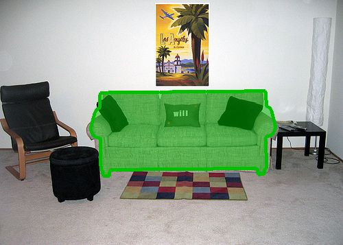
aeroplane      bicycle       boat       bottle        bus           car          chair      diningtable motorbike          sofa         train       tvmonitor        Avg.
DPM [6]                   42.2 / –      49.6 / –      6.0 / –    20.0 / –    54.1 / –      38.3 / –     15.0 / –       9.0 / –      33.1 / –      18.9 / –      36.4 / –      33.2 / –      29.6 / –
VDPM - 4V                40.0 / 34.6   45.2 / 41.7   3.0 / 1.5    –/–       49.3 / 26.1   37.2 / 20.2   11.1 / 6.8    7.2 / 3.1    33.0 / 30.4 6.8 / 5.1       26.4 / 10.7   35.9 / 34.7   26.8 / 19.5
VDPM - 8V                39.8 / 23.4   47.3 / 36.5   5.8 / 1.0    –/–       50.2 / 35.5   37.3 / 23.5   11.4 / 5.8    10.2 / 3.6   36.6 / 25.1 16.0 / 12.5     28.7 / 10.9   36.3 / 27.4   29.9 / 18.7
VDPM - 16V               43.6 / 15.4   46.5 / 18.4   6.2 / 0.5    –/–       54.6 / 46.9   36.6 / 18.1   12.8 / 6.0    7.6 / 2.2    38.5 / 16.1 16.2 / 10.0     31.5 / 22.1   35.6 / 16.3   30.0 / 15.6
VDPM - 24V                42.2 / 8.0   44.4 / 14.3   6.0 / 0.3    –/–       53.7 / 39.2   36.3 / 13.7   12.6 / 4.4    11.1 / 3.6   35.5 / 10.1 17.0 / 8.2      32.6 / 20.0   33.6 / 11.2   29.5 / 12.1
DPM-VOC+VP [21] - 4V 41.5 / 37.4 46.9 / 43.9         0.5 / 0.3    –/–       51.5 / 48.6   45.6 / 36.9   8.7 / 6.1     5.7 / 2.1    34.3 / 31.8   13.3 / 11.8   16.4 / 11.1   32.4 / 32.2   27.0 / 23.8
DPM-VOC+VP [21] - 8V 40.5 / 28.6 48.1 / 40.3         0.5 / 0.2    –/–       51.9 / 38.0   47.6 / 36.6   11.3 / 9.4    5.3 / 2.6    38.3 / 32.0   13.5 / 11.0   21.3 / 9.8    33.1 / 28.6   28.3 / 21.5
DPM-VOC+VP [21] - 16V 38.0 / 15.9 45.6 / 22.9        0.7 / 0.3    –/–       55.3 / 49.0   46.0 / 29.6   10.2 / 6.1    6.2 / 2.3    38.1 / 16.7    11.8 / 7.1   28.5 / 20.2   30.7 / 19.9   28.3 / 17.3
DPM-VOC+VP [21] - 24V 36.0 / 9.7 45.9 / 16.7         5.3 / 2.2    –/–       53.9 / 42.1   42.1 / 24.6   8.0 / 4.2     5.4 / 2.1    34.8 / 10.5    11.0 / 4.1   28.2 / 20.7   27.3 / 12.9   27.1 / 13.6
Table 2. The results of DPM, VDPM and DPM-VOC+VP are shown. The first number indicates the Average Precision (AP) for detection
and the second number shows the Average Viewpoint Precision (AVP) for joint object detection and pose estimation.

                                                                                                                                     0–1/3          1/3–2/3           2/3–max
original DPM, half of the mixture components are mirrored                                                      aeroplane              57.2            11.5              16.2
versions of the other half. So the training images are mir-                                                      bicycle              70.6            30.4               8.7
                                                                                                                  boat                13.1             0.7               0.9
rored and assigned to the mirror mixture components. Sim-                                                          bus                77.4            35.7               4.1
ilarly, we mirror the training images and assign them to the                                                       car                55.3            12.3               3.4
                                                                                                                  chair               22.0             7.5               0.9
mirrored viewpoint components in VDPM. Another way to                                                         diningtable             33.3            19.9               7.8
perform joint object detection and pose estimation is to treat                                                motorbike               56.5            12.6               0.1
                                                                                                                   sofa               35.3            34.2              15.8
it as a structure labeling problem. In Pepik et al. [21], they                                                    train               50.2            35.2              15.3
utilize structural SVM to predict the object bounding box                                                      tvmonitor              58.0             8.1               2.2
and pose jointly, where the model is called DPM-VOC+VP.                                                           Avg.                48.1            18.9               6.8
                                                                                                Table 3. The Normalized Average Precisions from VDPM with 8
In our baseline experiments, we divide the azimuth angles
                                                                                                views for object detection at different degrees of occlusion.
into 4, 8, 16 and 24 sections and train VDPM and DPM-
VOC+VP models for each case.
    To evaluate object detection, we use Average Precision                                      The detection performance of VDPM is on par with DPM.
(AP) as the metric and use the standard 50% overlap cri-                                        Compared with VDPM, DPM-VOC+VP achieves better
teria of PASCAL VOC [4]. For viewpoint estimation, the                                          viewpoint estimation in a tradeoff of slightly lower detec-
commonly used metric is the average over the diagonal of                                        tion performance. For most categories, as we increase the
the viewpoint confusion matrix [22]. However, this metric                                       number of viewpoints, the viewpoint estimation task be-
only considers the viewpoint accuracy among the correctly                                       comes harder and the AVP reduces, which is not surpris-
detected objects, which makes it non-comparable for two                                         ing. We can see from Table 2 that there is still a large room
detectors with different sets of detected objects. Since view-                                  for improvement both in detection and pose estimation on
point estimation is closely related to detection, we need a                                     our dataset. Hence, our 3D annotations can be valuable for
metric for joint detection and pose estimation. We propose a                                    developing new 3D object detection methods.
novel metric called Average Viewpoint Precision (AVP) for
this propose similar to AP in object detection. In computing                                    5.2. Sensitivity of Detection to Occlusion
AVP, an output from the detector is considered to be correct                                        Since our dataset provides occlusion labels for land-
if and only if the bounding box overlap is larger than 50%                                      marks, we can analyze the performance of detection at dif-
AND the viewpoint is correct (i.e., the two viewpoint labels                                    ferent degrees of occlusion. The occlusion of landmarks
are the same in discrete viewpoint space or the distance be-                                    does not directly determine the degree of occlusion of the
tween the two viewpoints is smaller than some threshold in                                      object, but it has a strong correlation with it. For exam-
continuous viewpoint space). Then we can draw a View-                                           ple, all landmarks can be occluded while most of the ob-
point Precision-Recall (VPR) curve similar to the PR curve.                                     ject can be observed, but such a case does not happen in
Average viewpoint precision is defined as the area under the                                    reality. Therefore, we use the ratio of externally occluded
VPR curve. Therefore, AVP is the metric for joint detection                                     or truncated landmarks to all landmarks as a measure for
and pose estimation. Note that detection PR curve is always                                     the degree of occlusion. We refer to it as the “occlusion
an upper bound of the VPR curve. Small gap between AVP                                          ratio”. In this experiment, we analyze the detection perfor-
and AP indicates high viewpoint accuracy among the cor-                                         mance of VDPM with 8 views in terms of different degree
rectly detected objects.                                                                        of occlusion. We partition the instances into three occlusion
   The results of the original DPM with 6 mixture com-                                          sets, i.e., the set with occlusion ratio between 0 and 1/3, the
ponents, VDPM and DPM-VOC+VP [21] for different az-                                             set with occlusion ratio between 1/3 and 2/3, and the set
imuth sections are shown in Table 2. Since the instances of                                     with occlusion ratio larger than 2/3. Since the number of
the bottle category are often symmetric across different az-                                    instances in each occlusion set is different, we report Nor-
imuth angles, it is ignored in VDPM and DPM-VOC+VP.                                             malized Average Precision in Table 3 as suggested by [10].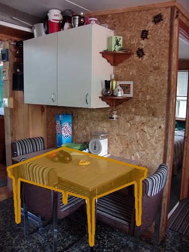
aeroplane bicycle boat bottle bus car chair diningtable motorbike sofa train tvmonitor Avg.
GT CAD 43.8 28.7 43.0 66.0 78.4 67.3 41.8 28.0 60.0 40.3 59.2 72.3 52.4
Random CAD 32.8± 0.3 29.2± 0.5 28.7± 1.1 62.5± 1.0 67.2± 0.8 61.8± 0.5 35.8± 0.8 21.3± 0.6 54.6± 0.3 34.7± 0.5 53.8± 0.6 60.5± 2.8 45.2
VDPM - 4 views 22.6 16.1 23.4 – 50.7 51.2 25.7 12.4 34.4 27.3 35.1 56.6 32.3
VDPM - 8 views 24.1 16.6 23.5 – 52.7 51.2 27.6 10.8 35.7 29.4 40.2 55.0 33.3
VDPM - 16 views 24.7 16.6 23.5 – 57.8 51.9 26.5 10.1 37.9 29.5 40.2 55.9 34.1
VDPM - 24 views 24.5 16.9 20.5 – 57.1 50.9 27.2 11.5 37.3 27.6 39.8 54.7 33.5
Table 4. Segmentation accuracy obtained by projecting the 3D CAD models onto the images. Please refer to the text for more details.
It is evident that the detectors have difficulty in handling We also evaluate how well the automatic approaches can
highly occluded objects. In order to achieve good perfor- perform segmentation. In this experiment, we infer the az-
mance in detection and pose estimation on our dataset, it is imuth automatically from VDPMs, but use the ground truth
important to handle the occluded and truncated objects. Our elevation, distance and CAD model in the projection. More
dataset enables evaluation of occlusion reasoning as well. specifically, for each detected object, we project the CAD
model to the image. We consider an object as detected
5.3. Segmentation using 3D Pose if there is a bounding box with more than 50% intersec-
We show that estimating the viewpoint with the corre- tion over union overlap associated with it. The performance
sponding CAD model for an object enables object segmen- drops significantly for the automatic approach. Note that the
tation. To find the upper bound for segmentation in this segmentation performance becomes better as we use finer
way, we project the ground truth CAD model (the one that discretization of azimuth (with the exception of 24 view-
the annotator selected for the object instance) onto the im- points). The low performance with 24 views might be due
age using the ground truth azimuth, elevation and distance. to the low performance of VDPM in viewpoint estimation
To evaluate the segmentation, we use the annotations pro- for 24 views as shown in Table 2.
vided by [9]. The first row of Table 4 shows the segmen-
tation accuracy using the ground truth poses, where we use 6. Conclusion
the standard PASCAL evaluation metric for segmentation.
The accuracy is not 100% due to several reasons. First, we To further improve the development of 3D object detec-
do not consider occlusion reasoning in the projection, and tion and pose estimation methods, we provide a large scale
the ground truth mask from [9] is just for the visible part of benchmark PASCAL3D+ with 3D annotations of objects.
the object. Second, due to the simplified camera model in PASCAL3D+ overcomes the limitations of the existing 3D
computing the continuous pose and the limited number of datasets and better matches real-world scenarios. We devel-
CAD models in our dataset, the projection matrix we use is oped an algorithm and annotation tool to provide the con-
an approximation to the real one. So we also include the tinuous 3D viewpoint annotations in unconstrained settings,
re-projection error in our 3D annotation, which can be con- where the camera parameters are unknown and only a sin-
sidered to be a measure for the quality of the annotation. gle image of object instances is available. We also provide
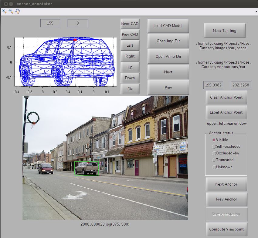
Figure 7 shows segmentation examples for each category in baseline results for object detection, viewpoint estimation
our dataset using the ground truth pose. As an example of and segmentation on our PASCAL3D+ dataset. The results
the re-projection error, the predicted legs of the diningtable illustrate that there is still a large room for improvement in
are not precisely aligned with the object in the image, which all these tasks. We hope our dataset can push forward the
results in a large penalty in the computing the segmentation research in 3D object detection and pose estimation.
accuracy. For the chairs, a large penalty is introduced due
to occlusion. Occlusion reasoning is also important for seg- Acknowledgments
mentation. We acknowledge the support of ONR grant N00014-13-
To show the importance of using the right CAD model 1-0761 and NSF CAREER grant #1054127. We thank Tae-
for annotation, instead of projecting the ground truth CAD won Kim, Yawei Wang and Jino Kim for their valuable help
model, we project a randomly chosen model (from the set in building this benchmark. We thank Bojan Pepik for his
of CAD models for a particular category) and evaluate the help in conducting the experiments with DPM-VOC+VP.
segmentation performance. As shown in the second row
of Table 4, the average accuracy drops by about 7%. The References
shown accuracy is the average over 5 different random se-
lections. Note that the performance for bicycle with random [1] Google 3D Warehouse. http://sketchup.google.com/
3dwarehouse.
models is higher than the case with the ground truth models.
[2] A. Ansar and K. Daniilidis. Linear pose estimation from points or
This is due to the inaccuracy in 2D segmentation annotation lines. In ECCV, 2002.
of bicycle. In most cases, the areas that correspond to the [3] J. Deng, W. Dong, R. Socher, L. Li, K. Li, and L. Fei-Fei. Imagenet:
background are labeled as bicycle (e.g., around the spokes). A large-scale hierarchical image database. In CVPR, 2009.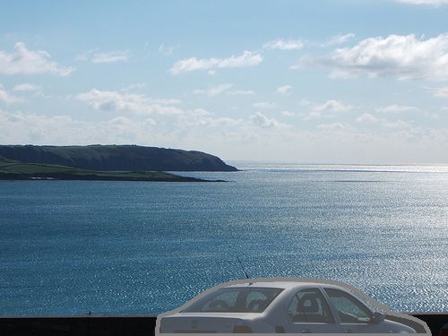
Figure 7. Segmentation results obtained by projecting the 3D CAD models to the images. Each figure shows an example for one of the 12
categories in our dataset.

 [4] M. Everingham, L. Van Gool, C. K. I. Williams, J. Winn, and A. Zis-             tated Real-world Objects. http://agamenon.tsc.uah.es/
     serman. The pascal visual object classes (voc) challenge. IJCV,                 Personales/rlopez/data/icaro, 2010.
     2010.                                                                    [17]   R. J. Lopez-Sastre, T. Tuytelaars, and S. Savarese. Deformable part
 [5] L. Fei-Fei, R. Fergus, and P. Perona. Learning generative visual mod-           models revisited: A performance evaluation for object category pose
     els from few training examples: an incremental bayesian approach                estimation. In ICCV Workshop on Challenges and Opportunities in
     tested on 101 object categories. In CVPR Workshop on Generative-                Robot Perception, 2011.
     Model Based Vision, 2004.                                                [18]   C. P. Lu, G. D. Hager, and E. Mjolsness. Fast and globally convergent
 [6] P. F. Felzenszwalb, R. B. Girshick, D. McAllester, and D. Ramanan.              pose estimation from video images. PAMI, 2000.
     Object detection with discriminatively trained part based models.        [19]   K. Matzen and N. Snavely. Nyc3dcars: A dataset of 3d vehicles in
     PAMI, 2010.                                                                     geographic context. In ICCV, 2013.
 [7] V. Ferrari, F. Jurie, and C. Schmid. From images to shape models for     [20]   M. Ozuysal, V. Lepetit, and P. Fua. Pose estimation for category
     object detection. IJCV, 2009.                                                   specific multiview object localization. In CVPR, 2009.
 [8] A. Geiger, P. Lenz, and R. Urtasun. Are we ready for autonomous          [21]   B. Pepik, M. Stark, P. Gehler, and B. Schiele. Teaching 3d geometry
     driving? the kitti vision benchmark suite. In CVPR, 2012.                       to deformable part models. In CVPR, 2012.
 [9] B. Hariharan, P. Arbelaez, L. Bourdev, S. Maji, and J. Malik. Seman-     [22]   S. Savarese and L. Fei-Fei. 3d generic object categorization, local-
     tic contours from inverse detectors. In ICCV, 2011.                             ization and pose estimation. In ICCV, 2007.
[10] D. Hoiem, Y. Chodpathumwan, and Q. Dai. Diagnosing error in              [23]   J. Shotton, J. Winn, C. Rother, and A. Criminisi. Textonboost for im-
     object detectors. In ECCV, 2012.                                                age understanding: Multi-class object recognition and segmentation
                                                                                     by jointly modeling appearance, shape and context. IJCV, 2007.
[11] A. Janoch, S. Karayev, Y. Jia, J. Barron, M. Fritz, K. Saenko, and
     T. Darrell. A category-level 3-d object dataset: Putting the kinect to   [24]   N. Silberman, D. Hoiem, P. Kohli, and R. Fergus. Indoor segmenta-
     work. In ICCV Workshop on Consumer Depth Cameras in Computer                    tion and support inference from rgbd images. In ECCV, 2012.
     Vision, 2011.                                                            [25]   M. Sun, G. Bradski, B.-X. Xu, and S. Savarese. Depth-encoded
                                                                                     hough voting for coherent object detection, pose estimation, and
[12] K. Lai, L. Bo, X. Ren, and D. Fox. A large-scale hierarchical multi-
                                                                                     shape recovery. In ECCV, 2010.
     view rgb-d object dataset. In ICRA, 2011.
                                                                              [26]   A. Thomas, V. Ferrari, B. Leibe, T. Tuytelaars, B. Schiele, and L. V.
[13] B. Leibe and B. Schiele. Analyzing appearance and contour based
                                                                                     Gool. Towards multi-view object class detection. In CVPR, 2006.
     methods for object categorization. In CVPR, 2003.
                                                                              [27]   Y. Xiang and S. Savarese. Estimating the aspect layout of object
[14] V. Lepetit, F. Moreno-Noguer, and P. Fua. Epnp: An accurate o(n)
                                                                                     categories. In CVPR, 2012.
     solution to the pnp problem. IJCV, 2009.
                                                                              [28]   J. Xiao, J. Hays, K. Ehinger, A. Oliva, and A. Torralba. Sun database:
[15] J. Lim, H. Pirsiavash, and A. Torralba. Parsing ikea objects: Fine              Large-scale scene recognition from abbey to zoo. In CVPR, 2010.
     pose estimation. In ICCV, 2013.
                                                                              [29]   J. Xiao, A. Owens, and A. Torralba. Sun3d: A database of big spaces
[16] R. J. Lopez-Sastre, C. Redondo-Cabrera, P. Gil-Jimenez, and                     reconstructed using sfm and object labels. In ICCV, 2013.
     S. Maldonado-Bascon.           ICARO: Image Collection of Anno-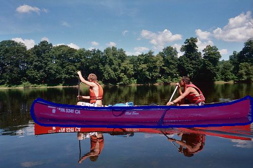
You can also read