Machine learning methods for the detection of polar lows in satellite mosaics: major issues and their solutions.
←
→
Page content transcription
If your browser does not render page correctly, please read the page content below
Machine learning methods for the detection of polar
                                                lows in satellite mosaics: major issues and their
                                                solutions.
arXiv:2011.04811v1 [physics.ao-ph] 9 Nov 2020

                                                             Mikhail Krinitskiy1 , Polina Verezemskaya1 , Svyatoslav Elizarov2 ,
                                                             Sergey Gulev1
                                                             E-mail: krinitsky@sail.msk.ru
                                                             1
                                                               Shirshov Institute of Oceanology, Russian Academy of Sciences, Moscow, Russia
                                                             2
                                                               Alterra.ai, Moscow, Russia

                                                             December 2019

                                                             Abstract. Polar mesocyclones (PMCs) and their intense subclass polar lows (PLs) are
                                                             relatively small atmospheric vortices that form mostly over the ocean in high latitudes.
                                                             PLs can strongly influence deep ocean water formation since they are associated with
                                                             strong surface winds and heat fluxes. Detection and tracking of PLs are crucial for
                                                             understanding the climatological dynamics of PLs and for the analysis of their impacts
                                                             on other components of the climatic system. At the same time, visual tracking of
                                                             PLs is a highly time-consuming procedure that requires expert knowledge and extensive
                                                             examination of source data.
                                                                 There are known procedures involving deep convolutional neural networks (DCNNs)
                                                             for the detection of large-scale atmospheric phenomena in reanalysis data that
                                                             demonstrate a high quality of detection. However, one cannot apply these procedures to
                                                             satellite data directly since, unlike reanalyses, satellite products register all the scales of
                                                             atmospheric vortices. It is also known that DCNNs were originally designed to be scale-
                                                             invariant. This leads to the problem of filtering of the scale of detected phenomena. There
                                                             are other problems to be solved, such as low signal-to-noise ratio of satellite data, and
                                                             an unbalanced number of negative (without PLs) and positive (where a PL is presented)
                                                             classes in a satellite dataset.
                                                                 In our study, we propose a deep learning approach for the detection of PLs and PMCs
                                                             in remote sensing data, which addresses class imbalance and scale filtering problems. We
                                                             also outline potential solutions for other problems, along with promising improvements
                                                             to the presented approach.

                                                1. Introduction

                                                Polar mesocyclones (PMCs) are high-latitude atmospheric vortices that form mostly over
                                                the ocean. PMCs are relatively small and short-living: their sizes vary from 200 to
                                                1000 km, and lifetime typically does not exceed 36 hours [1]. The intense subclass of
                                                PMCs, namely polar lows (PLs) characterizes by strong winds and high surface fluxes [2].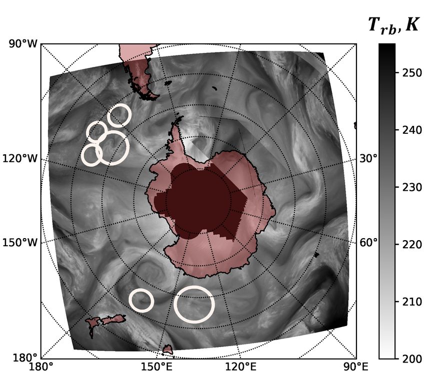
Despite their small sizes, PLs can cause rough seas and may deliver dangerous weather
conditions for engineering infrastructure, mostly due to their explosive formation and
unpredictable behavior. Moreover, PMCs and PLs were shown recently to influence ocean
convection, and deep water formation significantly [3–5]. Therefore, reliable identification
and tracking of PLs and PMCs are vital for their quantification as well as for assessing
their impact on the ocean circulation of various scales.
      The identification of PLs in atmospheric reanalyses is limited due to their sizes
compared to effective grid resolutions. The lack of representation of PMCs in modern
reanalyses was shown recently [1, 5–8]. As for reanalyses of high enough resolution,
the number of studies demonstrating PLs identification is still insufficient (e.g., [9]). In
some studies, automated mid-latitude cyclone tracking methods are applied to operational
analysis data with some adaptations to PL identification and tracking [10–12]. However,
the reported climatological characteristics such as the number of PLs, their sizes, their
lifetime vary significantly in these studies.
      Due to the lack of representation of PLs in reanalyses and operational analyses, in
our study, we focus on the detection of PLs in satellite imagery. Particularly, we use
satellite imagery of cloudiness for the identification of cloudiness patterns associated with
PLs. There are a number of studies exploiting the approach of manual identification and
tracking of PLs [1, 13–17], resulting in a comprehensive evaluation of characteristics of PLs
in various regions. However, the procedure of manual identification of PLs requires expert
knowledge and is enormously time-consuming. Thus, most of these studies are regional
and cover relatively short time periods. This approach is unacceptable in case one would
like to build a global long enough climatology of PLs. In this paper, we present further
development of the study presented in [18] which main goal is the automated method for
the identification and tracking of PLs in satellite data, which can reliably mimic a human
expert. This method will tackle the issue of high costs of PL identification.
      Machine learning (ML) and deep learning (DL), in particular, were shown recently to
be quite effective in problems related to pattern recognition, visual object detection, and
other computer vision tasks [19–23]. Some studies demonstrated successful applications
of DL methods in problems of the recognition of extreme weather events in reanalyses
[24–26]. However, most of the existing studies are focused on the detection of synoptic-
scale phenomena such as tropical cyclones or atmospheric rivers. DL methods were also
shown to be applicable in the problem of the detection of mesoscale and sub-mesoscale
oceanic eddies in SAR satellite imagery [27]. However, as of our best knowledge, there
are no applications of DL methods for the identification of PLs in satellite imagery.
      There are several reasons for this lack of studies: (i) A low signal-to-noise ratio of
satellite imagery limits the efficiency of most computer vision algorithms. (ii) Satellite
imagery preserves a full range of scales of atmospheric vortices, including synoptic
cyclones, MCs, and sub-mesoscale vortices, so the lack of the ability of scale filtering may
suppress the quality of an algorithm of PL detection. (iii) One of the most challenging
problems of DL applications in supervised problems in climate sciences is the lack of

                                             2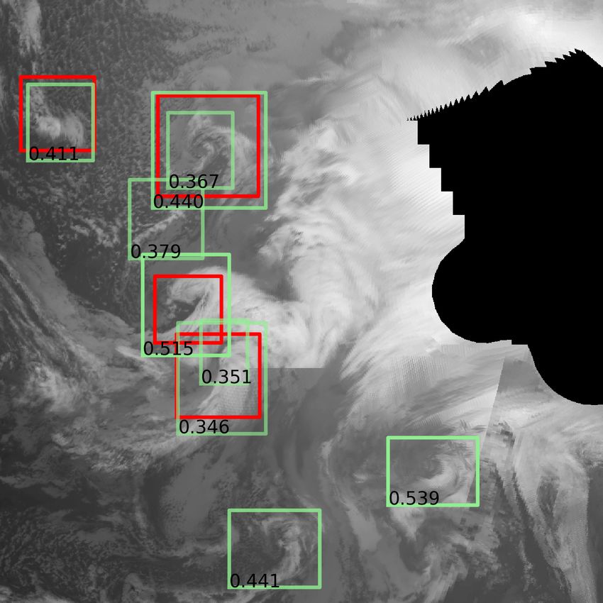
labeled datasets. While there are many well-established labeled datasets and benchmarks
for computer vision tasks [28–33], climate sciences are characterized by a huge amount of
unlabeled remote sensing data, reanalysis products, and model outputs. There are just a
few labeled datasets of PLs that may be used as supervision for DL models [1, 34, 35]. In
addition to the limited number of these catalogues, their sizes are small compared to the
number of labels typically needed for state of the art DL methods. (iv) Even in the case
of the dataset created with a consistent methodology applied to a homogeneous remote
sensing dataset [1], one has to deal with imbalanced labels meaning that the area occupied
by MCs (”positive” labels of imagery pixels) is low compared to the rest area (”negative”
labels of imagery pixels).
     Most of the mentioned issues do not impact the quality of the detection of large-scale
extreme weather events in reanalysis data (e.g., [24]). However, each of them has to be
addressed in case of the identification of PLs in satellite imagery.
     In this study, we present the novel method for the identification of PLs in satellite
imagery using a specific adaptation of an existing deep learning approach addressing the
issues of (a) labels imbalance; (b) scale filtering; (c) small labeled dataset. We also outline
further advances in our study, which may improve the quality of the detection.
     The rest of the paper is organized as follows: in section 2, we describe the source
data and the database of PLs we use; in section 3, we overview the preprocessing of
the source data and our method for the detection of PLs that we developed based on
deep convolutional neural networks (DCNN); in section 4, we present the results of the
application of our methodology. In section 5, we summarize the paper with the conclusions
and provide an outline of our further study.

2. Data

In this study, we used the database of PMCs in the Southern Ocean (SOMC, http:
//sail.ocean.ru/antarctica/) described in detail in [1]. The database contains
1735 MC tracks resulting in 9252 records of MC size, position, and cloudiness pattern
(according to the given in [17]). SOMC database covers the summer season of 2004 (June
to September). The trajectories of the database were built visually by an expert applying
the methodology described in [17]. The source data for this database were consecutive
three-hourly IR (10.3 − 11.3 microns) and WV (∼ 6.7 microns) satellite mosaics provided
by the Antarctic Meteorological Research Center (AMRC) - Antarctic Satellite Composite
Imagery (AMRC ASCI). The spatial resolution of the mosaics is 5 km, and temporal
resolution is 3 hours for the year 2004. AMRC ASCI mosaics cover the area to the South
of ∼ 40◦ S (see complete description in [36]).
     For the development of the detection algorithm, we processed the same AMRC ASCI
satellite imagery of IR and WV channels. We also included spatially and temporally
collocated sea level pressure (SLP) field of ERA-Interim reanalysis [37], which we
interpolated to the AMRC ASCI grid. SLP here essentially represents large-scale

                                              3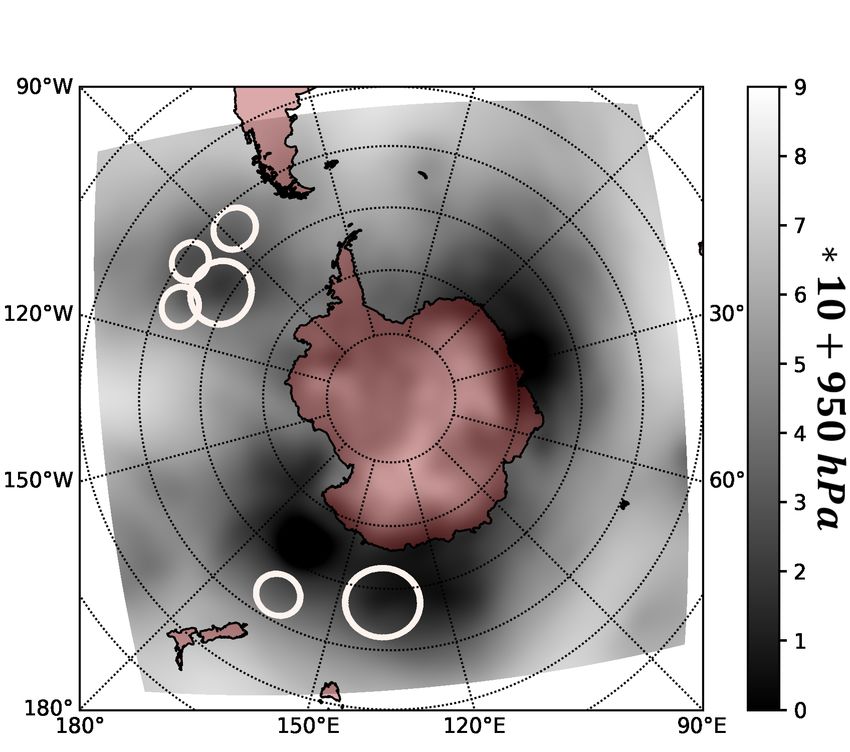
(a)                            (b)                           (c)

Figure 1: Source data at 2004-06-01 00:00 (UTC) for the detection of PLs: (a) IR mosaic,
(b) WV mosaic, and (c) SLP snapshot linearly downscaled to AMRC ASCI grid. The
white circles mark PLs identified by an expert in this snapshot.

circulation patterns e.g. synoptic cyclones, which one needs to filter out at the moment
of PLs detection. In fig. 1, one particular snapshot of source data is presented.

3. Method

The main problem of this study is to infer PLs positions and sizes, i.e., bounding boxes
of PLs (bboxes hereafter) for each time moment meaning in each 3-hourly source data
snapshot (see examples in fig. 2 shown by red squared bboxes).

3.1. Data preprocessing
First, we normalize the source data according to eq. 1:
                         x − xmin
              xnorm =               ,                                                 (1)
                        xmax − xmin
where x denotes IR, WV, or SLP fields; xmin and xmax are shown in the tab. 1. With this
normalization procedure, 99% of the values of normalized source data are in the range [0,
1]. All the values outside this range were masked and thus did not contribute to the loss
function of our DCNN model. Also, source satellite data comes with a mask that marks
the pixels where satellite data is missing or not usable.

                              Feature    xmin       xmax
                                 IR      200 K     300 K
                                WV       200 K     255 K
                                SLP     950 hPa   1040 hPa

                    Table 1: Normalizing coefficients for source data

                                           4
For the computational purpose, we cut sub-regions of source data of size 1024x1024
pixels for the training procedure of our DCNN. The size of one grid cell of AMRC ASCI
mosaics is ∼ 5 km, so the size of these cut regions is ∼ 5120 km, which is sufficient for
fitting any known PL. In fig. 2, examples of these sub-regions are shown. We perform
this sub-sampling procedure with the condition that each of these sub-regions contains at
least one PL bbox, and all the PL bboxes were present in these sub-regions completely. In
fig. 2, these ground truth labels (PL bboxes) introduced by a human expert are marked
by red bboxes.
We also apply data augmentation, which was shown to be helpful for DL models to
generalize better [23, 38–40]. In our study, we applied multiple augmentation techniques,
including Spatial Transform Networks [41] and Deep Diffeomorphic Transformer Networks
[42, 43]. We also employed a set of weak affine transformations using the python library
”imgaug” [44]. The augmentation was applied only to the train subset of data. As a
result, its amount increased significantly. In tab. 2, the number of augmented examples
is shown for the train set, as well as the numbers of non-augmented sub-region examples
and corresponding ground truth PL labels for validation and test sets.
Data subset No. of sub-regions No. of PL labels
train (augmented) 1009728 2466674
validation 12800 35252
test 9984 23482
Table 2: The number of cut sub-region examples and corresponding ground truth PL
labels in subsets of source data.
3.2. RetinaNet for the identification of PLs
In our study, we use the adaptation of the particular artificial neural network called
RetinaNet presented in [45]. This network is designed to perform the task of object
detection, which is precisely the case of PL identification.
The issue of unbalanced datasets is well known in ML and DL problems. There are
several ways to address this issue [46]. In the problem of the detection of PLs in satellite
imagery, it is barely possible to employ data-level methods (oversampling/undersampling).
Thus, the only option is classifier-level methods. In [45], cost-sensitive learning is
employed [46]. In particular, the novel loss function was introduced, namely focal loss
(FL hereafter, see eq. 2 for the α-balanced variant of FL).
F L(p̂) = −α(1 − p̂)γ ∗ log (p̂), (2)
where p̂ is an output of the network modeling a Bernoulli-distributed variable that is
commonly interpreted as an estimate of the probability of an object (enclosed with a
detected bbox) to have class ”1”, i.e., to be a PL in our study; α is a balancing parameter;
5γ is a focusing parameter of this loss function. FL was designed in replacement of the
commonly used cross-entropy loss to tackle the issue of highly imbalanced labels, which
is precisely the case in the problem of PL detection in satellite imagery. In this study,
we adjusted the value of γ = 3.5, which differs from the one proposed in [45]. This value
enforces the focus of our DCNN on positive labels.
The architecture of the model RetinaNet was originally presented in [45]. Apart
from the FL, a few novel approaches were implemented in RetinaNet. Among others, it
exploits transfer learning (TL) [47] with a backbone sub-network anticipatorily trained
on a large dataset like ImageNet [28]. In DL methods, TL addresses the lack of labeled
data. In our study, ResNet-152 [22] was employed as a backbone network. The authors
of RetinaNet empathize though that it achieves top results in object detection tasks not
based on innovations of the network design, but due to the novel loss function.
Following the established practice in visual object detection problems, we assess the
performance of PLs detection by mAP metric ([33]; higher is better; its values are in the
range [0, 1]). We also evaluated our adapted RetinaNet by mean intersection-over-union
(IoU , see eq. 1 in [33]) over all the detected PLs.
Following the approaches described in RetinaNet paper [45], we designed our
DCNN with the abovementioned adaptations regarding FL parameters and structural
particularities. The constructed DCNN based on RetinaNet was trained on the augmented
train subset. Quality assessment was performed on the test subset. For each of the
label proposals, the DCNN we constructed performs two tasks: (i) classification meaning
estimating the probability p̂ of the label proposal to enclose a PL, and (ii) regression
meaning adjusting the position and the size of the label proposal. Then we filter these
label proposals with the thresholding value pth . In our study, pth is a hyperparameter. We
optimized mean IoU w.r.t. pth using validation subset of data. We achieved the optimal
value pth = 0.34.
4. Results and discussion
In fig. 2, some examples of the application of the adapted RetinaNet are presented. As
one can see, qualitatively, our DCNN performs the PL detection task in good accordance
with ground truth. For example, in fig. 2b one can see an almost perfect match of detected
PLs with ground truth. In fig. 2c, all the PLs were identified; however, some false alarms
are presented. There are also a few PLs detected twice in the presented results.
With the pth optimized as mentioned in section 3.2, we assessed the quality of PLs
detection in terms of mean IoU and mAP : IoUmean = 0.27; mAP = 0.36. One may
argue that despite the good qualitative correspondence of identified PLs with expert-
defined labels, formal metrics are low compared to state of the art values (e.g., 0.869 in
[48]). However, there is a fundamental difference between a typical computer vision-based
object detection task and the task of PL detection. In a common visual object detection,
there are no concepts of the lifetime of objects, of the formation of objects or dissipation
6(a) (b) (c)
Figure 2: Results of the proposed detection model. Background shown with grayscale
color map represents IR normalized source data. Black areas represent the mask of missing
data. Ground truth labels are marked with red rectangles; detected PLs are marked with
green bounding boxes with the probability estimates p̂ indicated by text labels.
of objects. Thus, the comparison of mAP metric values with the best ones achieved with
state of the art DL approaches seems impractical.
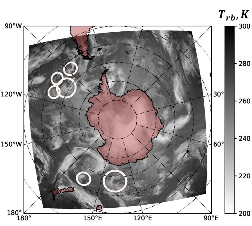
One of the main issues of PL detection problem compared to common object detection
is the need for conditioning of PL identification on its temporal evolution. For example,
consider fig. 3 with three consequent snapshots of source IR data. In fig. 3a, the detected
PLs (green bboxes) and expert-identified PLs (red bboxes) are presented; the same bboxes
in the same positions are shown in figures 3b and 3c for a reference. According to the
methodology [17], some of the detected cloudiness patterns may be interpreted as PLs.
However, these PL candidates dissipate quickly, so there are almost no signs of these
patterns in 3 and 6 hours. The lack of the proposed DCNN of consideration of temporal
evolution results in falsely detected PLs (false alarms). Currently, we consider this issue
as a major factor limiting the performance of our DCNN.
There are additional factors limiting the performance of the proposed method:
(a) in some cases of missing source data (shown with black regions in figures 2 and 3), an
expert may assume linear propagation of a PL through these regions, which results
in an additional PL label inside the masked region. Currently, there is no way to
implement or mimic this kind of decision in our method;
(b) the amount of labeled data in the PL detection problem is extremely insufficient
for the application of DL approaches to this problem. The abovementioned data
augmentation and transfer learning do improve the performance of the DCNN.
However, additional human expert labeling strongly required.
7(a) timestep t (b) timestep (t+3h) (c) timestep (t+6h)
Figure 3: An example of false PL detections: (a) detected and true labels at a time step
t; (b) the same labels at the same positions 3 hours after the time step t; (c) the same
labels at the same positions 6 hours after the time step t.
5. Conclusions and outlook
In this paper, a novel method for the identification of PLs in satellite mosaics is presented.
This method is based on a DCNN named RetinaNet, which was proposed for the visual
object detection task. As of our best knowledge, it is the first application of deep
convolutional neural networks to the problem of the detection of PLs and PMCs in satellite
mosaics data. In this study, RetinaNet and FL were adapted to the specifics of the problem
of PL detection. In particular, focusing parameter γ of the FL was set to a higher value
in order to make the DCNN more focused on positive labels that denote the bboxes
where PLs are presented. With this approach, we address the issue of class imbalance.
The source data for the identification of PLs were satellite mosaics of AMRC ASCI. We
also included spatially and temporally collocated SLP fields from ERA-Interim reanalysis
in order to address the issue of scale filtering since SLP essentially encodes large scale
atmospheric circulation.
There are several approaches we intend to apply further. The most promising
modification of the proposed model is a new neural network architecture that takes
the temporal evolution of multiscale atmospheric circulation into account. There are
additional modifications of the method, which may improve the quality of the detection.
One of them is the regularization of the model, which constrains the geometric parameters
of label bboxes. One more potential improvement implies the development of the SOMC
database. The promising approach here is to use assisted labeling. Since there is already a
model presented in this study that detects PLs and PMCs with some noise, it is promising
to use it for generating noisy PL proposals. For a human expert, binary classification (”it
is a PL”/”it is not a PL”) of the proposed labels is much faster compared to an extensive
examination of the whole source data example. This approach makes it possible to address
the major deep learning issue of insufficient labeled datasets.
86. Acknowledgements
This work was undertaken with financial support by the Russian Ministry of Science and
Higher Education (agreement №05.616.21.0112), project ID RFMEFI61619X0112)
References
[1] Verezemskaya P, Tilinina N, Gulev S, Renfrew IA, Lazzara M. Southern Ocean
mesocyclones and polar lows from manually tracked satellite mosaics. Geophysical Research
Letters. 2017 Aug; 44(15):7985–7993.
[2] Rasmussen EA, Turner J, editors. Polar Lows: Mesoscale Weather Systems in the Polar
Regions. Cambridge: Cambridge University Press ; 2003.
[3] Marshall J, Schott F. Open-ocean convection: Observations, theory, and models. Reviews
of Geophysics. 1999 Feb; 37(1):1–64.
[4] Condron A, Bigg GR, Renfrew IA. Modeling the impact of polar mesocyclones on ocean
circulation. Journal of Geophysical Research: Oceans. 2008; 113(C10).
[5] Condron A, Renfrew IA. The impact of polar mesoscale storms on northeast Atlantic Ocean
circulation. Nature Geoscience. 2013 Jan; 6(1):34–37.
[6] Laffineur T, Claud C, Chaboureau JP, Noer G. Polar Lows over the Nordic Seas: Improved
Representation in ERA-Interim Compared to ERA-40 and the Impact on Downscaled
Simulations. Monthly Weather Review. 2014 Jan; 142(6):2271–2289.
[7] Michel C, Terpstra A, Spengler T. Polar Mesoscale Cyclone Climatology for the Nordic
Seas Based on ERA-Interim. Journal of Climate. 2017 Dec; 31(6):2511–2532.
[8] Bromwich DH, Wilson AB, Bai LS, Moore GWK, Bauer P. A comparison of the regional
Arctic System Reanalysis and the global ERA-Interim Reanalysis for the Arctic. Quarterly
Journal of the Royal Meteorological Society. 2016 Jan; 142(695):644–658.
[9] Gavrikov A, Gulev S, Markina M, Tilinina N, Verezemskaya P, Barnier B, et al. RAS-
NAAD: 40-year high resolution North Atlantic atmospheric hindcast for multipurpose
applications (new dataset for the regional meso-scale studies in the atmosphere and the
ocean). Journal of Applied Meteorology and Climatology. , in review;.
[10] Zappa G, Shaffrey L, Hodges K. Can Polar Lows be Objectively Identified and Tracked in
the ECMWF Operational Analysis and the ERA-Interim Reanalysis? Monthly Weather
Review. 2014 Apr; 142(8):2596–2608.
[11] Pezza A, Sadler K, Uotila P, Vihma T, Mesquita MDS, Reid P. Southern Hemisphere
strong polar mesoscale cyclones in high-resolution datasets. Climate Dynamics. 2016 Sep;
47(5-6):1647–1660.
[12] Xia L, Zahn M, Hodges K, Feser F, Storch H. A comparison of two identification and
tracking methods for polar lows. Tellus A: Dynamic Meteorology and Oceanography. 2012
Dec; 64(1):17196.
[13] Harold JM, Bigg GR, Turner J. Mesocyclone activity over the North-East Atlantic. Part
1: vortex distribution and variability. International Journal of Climatology. 1999 Sep;
19(11):1187–1204.
9[14] Harold JM, Bigg GR, Turner J. Mesocyclone activity over the Northeast Atlantic. Part
2: An investigation of causal mechanisms. International Journal of Climatology. 1999 Oct;
19(12):1283–1299.
[15] Carrasco JF, Bromwich DH, Liu Z. Mesoscale cyclone activity over Antarctica during
1991: 1. Marie Byrd Land. Journal of Geophysical Research: Atmospheres. 1997 Jun;
102(D12):13923–13937.
[16] Turner J, Thomas JP. Summer-season mesoscale cyclones in the bellingshausen-weddell
region of the antarctic and links with the synoptic-scale environment. International Journal
of Climatology. 1994 Oct; 14(8):871–894.
[17] Carleton AM. On the interpretation and classification of mesoscale cyclones from satellite
infrared imagery. International Journal of Remote Sensing. 1995 Sep; 16(13):2457–2485.
[18] Krinitskiy M, Verezemskaya P, Grashchenkov K. Convolutional neural networks for
Antarctic mesocyclones identification using satellite mosaics data. In: Geophysical Research
Abstracts. vol. 20; 2018. p. EGU2018–17631.
[19] Lin TY, Dollár P, Girshick R, He K, Hariharan B, Belongie S. Feature Pyramid Networks
for Object Detection. arXiv:161203144 [cs]. 2016 Dec; ArXiv: 1612.03144.
[20] Simonyan K, Zisserman A. Very Deep Convolutional Networks for Large-Scale Image
Recognition. arXiv:14091556 [cs]. 2014 Sep; ArXiv: 1409.1556.
[21] Badrinarayanan V, Kendall A, Cipolla R. SegNet: A Deep Convolutional Encoder-Decoder
Architecture for Image Segmentation. arXiv:151100561 [cs]. 2015 Nov; ArXiv: 1511.00561.
[22] He K, Zhang X, Ren S, Sun J. Deep Residual Learning for Image Recognition;. p. 770–778.
[23] Krizhevsky A, Sutskever I, Hinton GE. ImageNet Classification with Deep Convolutional
Neural Networks. In: Pereira F, Burges CJC, Bottou L, Weinberger KQ, editors. Advances
in Neural Information Processing Systems 25. Curran Associates, Inc.; 2012. p. 1097–1105.
[24] Liu Y, Racah E, Prabhat, Correa J, Khosrowshahi A, Lavers D, et al. Application of
Deep Convolutional Neural Networks for Detecting Extreme Weather in Climate Datasets.
arXiv:160501156 [cs]. 2016 May; ArXiv: 1605.01156.
[25] Muszynski G, Kashinath K, Kurlin V, Wehner M, Prabhat. Topological data analysis
and machine learning for recognizing atmospheric river patterns in large climate datasets.
Geoscientific Model Development. 2019 Feb; 12(2):613–628.
[26] Rupe A, Kashinath K, Kumar N, Lee V, Prabhat, Crutchfield JP. Towards Unsupervised
Segmentation of Extreme Weather Events. arXiv:190907520 [physics]. 2019 Sep; ArXiv:
1909.07520.
[27] Huang D, Du Y, He Q, Song W, Liotta A. DeepEddy: A simple deep architecture for
mesoscale oceanic eddy detection in SAR images. In: 2017 IEEE 14th International
Conference on Networking, Sensing and Control (ICNSC); 2017. p. 673–678.
[28] Deng J, Dong W, Socher R, Li LJ, Li K, Fei-Fei L. Imagenet: A large-scale hierarchical
image database. In: Computer Vision and Pattern Recognition, 2009. CVPR 2009. IEEE
Conference on. Ieee; 2009. p. 248–255.
[29] Krizhevsky A. Learning multiple layers of features from tiny images. University of Toronto;
2009.
[30] Lecun Y, Bottou L, Bengio Y, Haffner P. Gradient-based learning applied to document
recognition. Proceedings of the IEEE. 1998 Nov;86(11):2278–2324.
10[31] Cordts M, Omran M, Ramos S, Rehfeld T, Enzweiler M, Benenson R, et al. The Cityscapes
Dataset for Semantic Urban Scene Understanding. arXiv:160401685 [cs]. 2016 Apr; ArXiv:
1604.01685.
[32] Lin TY, Maire M, Belongie S, Bourdev L, Girshick R, Hays J, et al. Microsoft COCO:
Common Objects in Context. arXiv:14050312 [cs]. 2015 Feb; ArXiv: 1405.0312.
[33] Everingham M, Eslami SMA, Van Gool L, Williams CKI, Winn J, Zisserman A. The Pascal
Visual Object Classes Challenge: A Retrospective. International Journal of Computer
Vision. 2015 Jan; 111(1):98–136.
[34] Noer G, Lien T. Dates and Positions of Polar lows over the Nordic Seas between 2000 and
2010. Norwegian Meteorological Institute Rep. 2010;.
[35] Noer G, Saetra O, Lien T, Gusdal Y. A climatological study of polar lows in the Nordic
Seas. Quarterly Journal of the Royal Meteorological Society. 2011 Oct; 137(660):1762–1772.
[36] Kohrs RA, Lazzara MA, Robaidek JO, Santek DA, Knuth SL. Global satellite composites
— 20 years of evolution. Atmospheric Research. 2014 Jan; 135-136:8–34.
[37] Dee DP, Uppala SM, Simmons AJ, Berrisford P, Poli P, Kobayashi S, et al. The
ERA-Interim reanalysis: configuration and performance of the data assimilation system.
Quarterly Journal of the Royal Meteorological Society. 2011; 137(656):553–597.
[38] Dosovitskiy A, Fischer P, Springenberg JT, Riedmiller M, Brox T. Discriminative
Unsupervised Feature Learning with Exemplar Convolutional Neural Networks. IEEE
Transactions on Pattern Analysis and Machine Intelligence. 2016 Sep;38(9):1734–1747.
[39] Zeiler MD, Fergus R. Visualizing and Understanding Convolutional Networks. In: Fleet D,
Pajdla T, Schiele B, Tuytelaars T, editors. Computer Vision – ECCV 2014. Lecture Notes
in Computer Science. Cham: Springer International Publishing; 2014. p. 818–833.
[40] Howard AG. Some Improvements on Deep Convolutional Neural Network Based Image
Classification. arXiv:13125402 [cs]. 2013 Dec; ArXiv: 1312.5402.
[41] Jaderberg M, Simonyan K, Zisserman A, Kavukcuoglu K. Spatial Transformer Networks.
arXiv:150602025 [cs]. 2016 Feb; ArXiv: 1506.02025.
[42] Skafte Detlefsen N, Freifeld O, Hauberg S. Deep Diffeomorphic Transformer Networks;
2018. p. 4403–4412.
[43] Freifeld O, Hauberg S, Batmanghelich K, Fisher JW. Transformations Based on Continuous
Piecewise-Affine Velocity Fields. IEEE Transactions on Pattern Analysis and Machine
Intelligence. 2017 Dec;39(12):2496–2509.
[44] Jung AB, Wada K, Crall J, Tanaka S, Graving J, Yadav S, et al.. imgaug; 2019. Online;
accessed 25-Sept-2019. https://github.com/aleju/imgaug.
[45] Lin TY, Goyal P, Girshick R, He K, Dollar P. Focal Loss for Dense Object Detection; 2017.
p. 2980–2988.
[46] Buda M, Maki A, Mazurowski MA. A systematic study of the class imbalance problem in
convolutional neural networks. Neural Networks. 2018 Oct; 106:249–259.
[47] Kolesnikov A, Beyer L, Zhai X, Puigcerver J, Yung J, Gelly S, et al. Large Scale Learning
of General Visual Representations for Transfer. arXiv:191211370 [cs]. 2019 Dec; ArXiv:
1912.11370.
[48] Singh B, Najibi M, Davis LS. SNIPER: Efficient Multi-Scale Training. arXiv:180509300
[cs]. 2018 Dec; ArXiv: 1805.09300 version: 3.
11You can also read