Object detection for crabs in top-view seabed imagery
←
→
Page content transcription
If your browser does not render page correctly, please read the page content below
Object detection for crabs in top-view seabed imagery

                                                             Vlad Velici                                Adam Prügel-Bennett
                                            School of Electronics and Computer Science        School of Electronics and Computer Science
                                                    University of Southampton                         University of Southampton
                                                         Southampton, UK                                   Southampton, UK
arXiv:2105.02964v1 [cs.CV] 2 May 2021

                                                                                      Abstract

                                                 This report presents the application object detection on a database of underwater
                                                 images of different species of crabs, as well as aerial images of sea lions and Pascal
                                                 VOC. The model is an end-to-end object detection model based on a convolutional
                                                 network and a Long Short-Term Memory detector.

                                        1     Introduction

                                        This report presents the problem of object detection and classification, popular datasets, and in
                                        Section 1.1 we present the datasets relevant to this work.
                                        Image classification is the task of labelling an image with a class. Given an input image a model
                                        must predict what class it belongs to. Images used for classification often have one large central
                                        object. However this is not the case in real life where we are surrounded by many objects. A more
                                        challenging task is to predict where all the objects are in an image and what class they belong to. We
                                        call this object detection. An intermediary objective can be object localisation which is simply the
                                        task of finding all objects in an image but not assigning a class to them.
                                        Depending on the actual dataset and desired end result, an object is defined by its class and either
                                        its x and y coordinates or a bounding box (x, y coordinates, width w and height h). We will use the
                                        term object coordinates to refer to either x and y coordinates or a bounding box.
                                        Datasets like PASCAL Visual Object Classes (object detection challenge) (Everingham et al., 2015)
                                        and COCO (Lin et al., 2014) have bounding box coordinates, where other datasets like the ones used
                                        in the NOAA Fisheries Steller Sea Lion Population Count Kaggle competition (NOAA Fisheries,
                                        2017) and the data obtained from (Thornton et al., 2016) only have the centre coordinate of the
                                        objects. Semantic segmentation is a type of object detection where the bounding boxes or coordinates
                                        are replaced with object boundaries at pixel level. We are not looking into semantic segmentation in
                                        this report at this time.

                                        1.1   Crabs and Steller Sea Lions datasets

                                        Steller Sea Lion population started to decline in the 1970s, and in 1990 it was listed as a threatened
                                        species. NOAA Fisheries divided the population into the western stock and the eastern stock, the
                                        separation line being at 144 deg West longitude. The eastern stock population started to recover in
                                        the late 1970s and has fully recovered in 2013. However, the western stock population has not. The
                                        population in the eastern side of the western stock (144 deg - 170 deg West longitude) is increasing,
                                        but the western end, in Aleutian Islands, continues to decline. A map of the locations can be seen
                                        in Figure 1. NOAA Fisheries is working on creating long-term population trends over time to help
                                        develop recovering strategies for the endangered population. Having such trends and tools will allow
                                        NOAA to make better decisions about managing fisheries and to identify possible threats affecting
                                        the endangered populations (Fritz et al., 2016).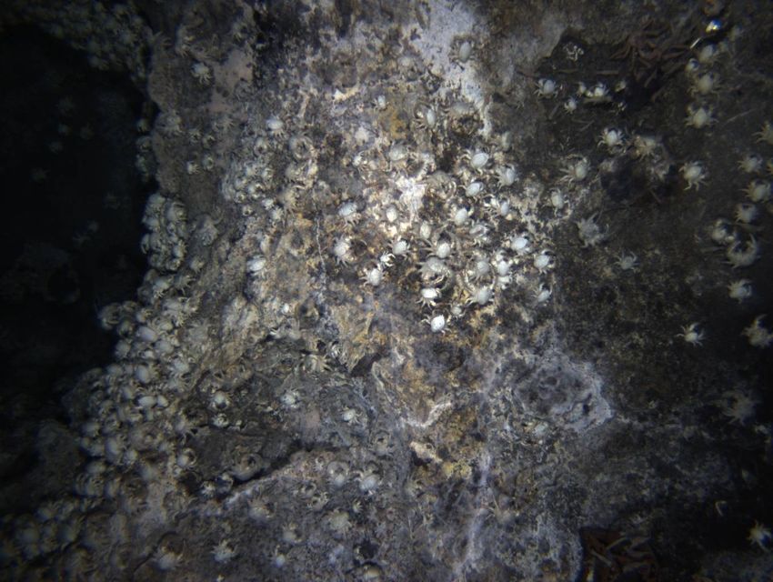
Figure 1: Map of Steller Sea Lion populations from NOAA Fisheries outreach video https://youtu.
be/oiL8tDCqzy4. Red area shows the endangered population, yellow area shows the population
that is increasing and green area shows the population that has fully recovered in 2013.

NOAA Fisheries can now gather large amounts of aerial imagery efficiently using drones. They are,
however, facing the problem of manually labelling the images to be able to create population trends.
Currently they use human labelling but this method is prone to errors and slow, thus they are seeking
automated solutions to improve the speed and quality of labelling. They have launched a Kaggle1
competition to invite data scientists to find solutions and implement models to solve the labelling
problem. The competition has a dataset of 100+GB of labelled imagery (NOAA Fisheries, 2017).
The work presented in Thornton et al. (2016) is a practical method of using underwater robots to
survey large areas of seafloor (multi-hectare areas). The images produced were then processed to build
3D reconstructions and mosaics which were manually labelled for 6 taxa of animals (crabs, mussels
and shrimps). Labelling taxa by hand is a long, slow, expensive and error prone process, and it is the
bottleneck of the whole process of creating population densities and distributions efficiently. They
produced a dataset of two labelled mosaics of imagery taken at two locations: C0014G_2m_2014 is a
1060m deep drill site in the Iheya North field, and NBC_2m_2014 is a naturally active site located
500m away.
In this report we will present a model created for these two datasets and report its performance,
training and possible improvements.

1.1.1      Note on the state of the art

This work was part of my PhD initial project, which was done in 2016, for the purpose of exploring
deep learning and object detection, not necessarily to obtain good results. If the reader is interested in
exploring the field of object detection and building competitive models we suggest to look up the
current state of the art models and methods. We refrain from mentioning any works here because
they will quickly become out of date.

2       Crab detector network

In this report we present a deep neural network built for end-to-end object detection. As an end-to-end
model, it takes as an input an image and outputs object coordinates, classes and confidence scores.
The model can be configured to use centre coordinates of the objects or bounding boxes.

    1
        Kaggle: https://kaggle.com/

                                                    2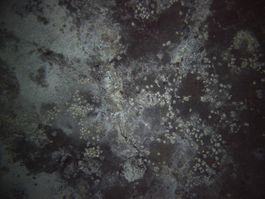
LSTM               Dense            Relative
                                                                                  (sigmoid)          x, y, w, h

                                                                 LSTM               Dense            Confidence
                                                                                  (sigmoid)          (objectness)
                                                                   ...
                                                                                    Dense            Class
                                                                                  (softmax)          probabilities
                                                                 LSTM

                                                                            For every grid cell, for every LSTM
      Input image      Convolutional layers   Feature map      RNN Layers   timestep.
                                                 (grid)

                                    Figure 2: Architecture of our model.

The model is built for the crabs and sea lions datasets where objects are defined by centre coordinates
and are relatively small but it is also evaluated on VOC12 where objects are described by bounding
boxes.

3   Model architecture

The model architecture is based on Stewart et al. (2016). We improved on their model by adding a
classifier and adapting the loss function. We also added support for x, y coordinates labels as well as
bounding boxes to enable using the model on the Pascal VOC 2012 dataset, the crabs and the Steller
Sea Lions datasets.
The model architecture is illustrated in Figure 2. For a forward pass, the model performs the following
steps:
Step 1 The input image is fed into a Convolutional Neural Network (CNN). The feature map that
results from the CNN is a B × W × H × F grid, where B is the batch size, W, H are the width and
height of the grid and F is the number of filters in the last convolutional layer.
Step 2 Each of the B × W × H grid cells (F -sized feature vectors) is fed into a layer of Long
Short-Term Memory cells (LSTMs). Note that changes in W and H can be considered changes in
the batch size B, therefore the model can be used for any input image size.
Step 3 At each recurrence the LSTM cells are densely connected to three different units: one to
predict objectness (used as confidence score), one to predict class probabilities (softmax), and one to
predict object coordinates relative to the centre of the grid cell.
For our experiments we use square input images of 224 × 224 pixels, therefore our grid is a square of
size G = W = H. We use two CNN configurations that result in G = 7 and G = 4, respectively.
Although we use a fixed image size as input, the model can support input images of any size as
the LSTM and dense layers receive a fixed-size input regardless of the input image size. The grid
size changes with the input image and affects how many times the LSTM and dense layers are run
sequentially across the image.
A fixed number of recurrences (time steps) of the LSTM cells, k, is set. This is an implementation
limitation. Theoretically, at test time the model can run recurrences until a stop symbol is produced
(first object with confidence below a set threshold, e.g. 0.5). During training the model can have one
recurrence for each ground truth label and an additional one for training the stop symbol. This can be
used to speed up the computations.
There is no ground truth order in which the objects in an image must be predicted. Therefore simply
matching predictions and ground truth labels as they appear would induce errors if the order does not
match. For instance, if an image has objects A and B given in the ground truth labels in this order
and the model predicts B, A, a direct matching would consider this prediction wrong, but in reality it
is correct. As suggested by Stewart et al. (2016), the Hungarian method is used as an efficient way to
match ground truth labels to predictions using the distance between the coordinates as the matching
cost.

                                                        3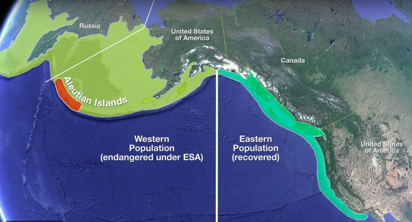
A new loss function was derived based on Stewart et al. (2016) and Redmon et al. (2016). The
loss function l is the sum of three components: the confidence (objectness) loss lo , the coordinates
(regression) loss lr and the class loss lc .
For the following equations we consider the ground truth labels to be sorted such that the ith element
of predictions is matched to the ith element of ground truth labels by the Hungarian method as
described above.
The confidence score prediction is designed as a binary classification problem and we use softmax
and cross-entropy loss for lo .
The regression loss is a root mean squared error function that only penalises predictions where
there is a real object. Define go to be the vector of ground truth confidence scores with elements
go (1), . . . , go (n) ∈ {0, 1} where n = G2 ∗ k is the number
                                                            Pn of predictions per image and go (i) = 1
if the prediction i is an object, 0 otherwise. Let m = i=1 go (i) be the number of real objects in
the image, Fr to be a n × r matrix, where r is the number of coordinates required per object (r = 2
for x, y coordinates and r = 4 for bounding boxes) with elements Fr (i, j) representing predicted
coordinates. Similarly, let Gr be a matrix of the same size with elements containing ground truth
coordinates or zeros if there is no object. We now define the regression loss
                                   v
                                   u        n          r
                                   u 1 X              X
                              lr = t           go (i)     (Fr (i, j) − Gr (i, j))2 .               (1)
                                     m ∗ r i=1        j=1

Let Fc be a n × C matrix (C is the number of classes) with rows Fc (i) representing the probabilities
of each class for object i (output of softmax). Similarly let Gc be a similar matrix representing the
ground truth. The class loss is
                                           n
                                        1 X
                                 lc =        go (i)H(Fc (i), Gc (i)),                             (2)
                                       m i=1
where H(a, b) is the cross-entropy between a and b. Note this is the cross-entropy loss but it only
penalises predictions where there is a real object (otherwise ground truth data does not exist for the
class).

4     Preprocessing
The labels are pre-processed such that, for an image, we will have G × G × k object labels in total,
k for each grid cell. If there are more than k objects in a particular grid cell, we cap them at k and
drop the rest. Less than 10 objects are dropped in the whole crabs dataset for k = 8. Objects with
confidence 0 are appended if there are fewer than k labels.
Label coordinates are made relative to the centre of the grid cell. We say the top left corner of a grid
cell is the point (0, 0) and the bottom right corner is the point (1, 1). The centre of the grid cell is
at (0.5, 0.5). This forces the LSTMs to predict objects that belong to their grid cell and makes the
network easier to train. In the case of bounding boxes, the width and height are relative to the input
image size, such that an object with width and height 1 covers the whole input image. This allows the
network to predict objects that are larger than a grid cell.
The image pixel values are normalised to fall between -0.5 and 0.5.

4.1   Crabs dataset

The crab dataset from Thornton et al. (2016) is made of two big mosaics C0014G_2m_2014 (20320 ×
28448 pixels) and NBC_2m_2014 (20320×20320 pixels), each representing an imaging location. We
slice the mosaics into 224 × 224 pixels images and randomly split them into training, cross-validation
(dev) and test sets (60% − 20% − 20%).
The labels consist of manually labelled x and y coordinates of each individual and its species.
The dataset is heavily unbalanced, as seen in Table 1. This leads to hard to train models thus we split
the dataset into two sub-datasets. We call crabs the dataset containing all images and crabs-top3 the
dataset consisting of the top 3 species by population count.

                                                   4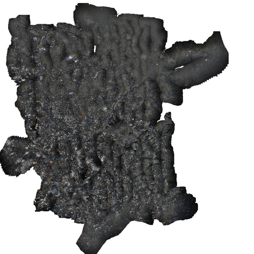
Table 1: Crabs species counts in the two locations (mosaics) and overall. The last column shows
which species are in the crabs-top3 dataset.
              Species                      C0014 NBC         Total    crabs-top3
              Alvinocaridid                   170    500       670
              Bathymodiolus japonicus 6,780         7,339 14,119            X
              Bathymodiolus platifrons 7,282 12,969 20,251                  X
              Paralomis                        96    109       205
              Shinkaia crosnieri             3,536  7,160 10,696            X
              Thermosipho desbruyesi           12     6         18
              Total individuals            17,876 28,083 45,959           45,066

Table 2: Sea Lions dataset population counts, showing the differences between the given population
counts and the generated dots. The dots have 16,955 dots that could not reliably be classified by
colour (not shown).
                                        Label counts Dot counts ∆
                     adult_males        5,392           5,349          43
                     subadult_males 4,345               4,028          317
                     adult_females      37,537          59,080         21,543
                     juveniles          20,118          20,895         777
                     pups               16,285          16,141         144
                     Totals             83,677          105,493        21,816

The big mosaics provided suffer from image quality loss as they are composed of individual higher-
quality images, overlapped and transformed to form a map-like mosaic. The effect can be observed
in Figure 3. The original images are available but, unfortunately, there is no mapping between the
labels on the mosaic and the original images, which are unlabelled.
Sequentially slicing the mosaics results in a total of 2608 224 × 224 images. A dataset of such a
small size is likely to make models easily overfit and hard to generalise. To address this issue we
heavily augment the training set with random rotations, zooms, shears, and shifts and also use a
different slicing technique where we cut an image centred on a crab. This results in a total of 45959
images (17,876 from C0014G and 28,083 from NBC) that have plenty of overlapping content.

4.2   Sea Lions dataset

The Steller Sea Lions dataset from the NOAA Kaggle competition (NOAA Fisheries, 2017) has many
large aerial images. 948 for training and 18,636 for testing during the competition. Similarly to the
crabs dataset, the dataset has x, y and class coordinates as labels, manually labeled.
The labels are given in two ways. Population counts per image are given in a CSV file. The x, y
coordinates are given in a second pair of training images annotated with coloured dots, the colour
denoting the class. The coordinates and classes can be extracted by subtracting the dotted and the pair
non-dotted training image and running a blob detector on the result. However, this pre-processing
step is a rather big source of errors in the training data used for our model. Population counts from
the CSV and the extracted dotted images are shown in Table 2.
The given training images are large (sizes 3744x5616, 4992x3328 and 5616x3744). We slice them
into 224x224 input images for training and testing. We split the given training set into a training and
dev set (80%-20%). The resulting dataset has 21,683 images for training and 5243 for dev.
The competition goal, and evaluation criteria, is the final population counts per image rather than
predicting where each individual is in the image.

5     Training and evaluation

A set of model configurations and hyper-parameters were chosen to train and evaluate our network
with. The CNN used to create a feature map is arguably the most important configuration choice.

                                                  5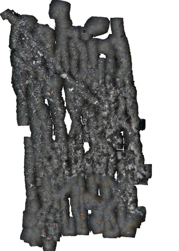
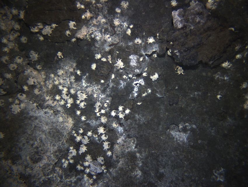
(a) Examples of original images from the crabs dataset.

         (b) The two mosaics of the crabs dataset. Left: C0014G_2m_2014, right: NBC_2m_2014.

(c) Two close-ups in the mosaics highlighting the effects of image quality loss, likely due to overlapping and
image processing for creating the mosaic.
Figure 3: Representation of the crabs dataset with example original images, the map mosaics from
which the training data is sliced and highlights of image quality loss in the mosaics.
                                                   6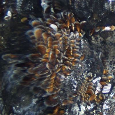
Table 3: Model evaluation on the crabs dataset with all classes used. 7x7 and 4x4 denote the grid
sizes used and slicing states the method of slicing the mosaics into training images. For slicing
around objects, the training set is based on the NBC mosaic, the dev set on C0014G and the test set is
sequentially sliced. Class values show AP %, mAP in %.
                                            Sliced sequentially                                Sliced around objects
                                     4x4                           7x7                     4x4                       7x7
                            Train    Dev       Test    Train       Dev     Test   Train    Dev     Test    Train     Dev    Test
 Bathymodiolus japonicus    61.12   36.81     38.50    12.41      10.02   10.38   71.00   41.63 22.46 46.65 9.27            9.26
 Thermosipho desbruyesi      9.17    9.29      9.19    46.74      28.91   32.53   26.08    9.11    9.12 55.51 25.87        18.08
 Bathymodiolus platifrons   60.81   40.81     33.27    52.34      28.65   31.01   75.59   36.14 20.59 61.33 30.38          17.89
 Paralomis                  12.49   10.02      9.59    11.74       9.48    9.54   14.89    9.30    9.72 20.72 9.15          9.24
 Alvinocaridid              11.98   10.30     11.04    50.82      30.34   23.37   46.43    9.81    9.71 60.18 28.05        16.38
 Shinkaia crosnieri         56.61   39.71     43.27     9.12       9.10    9.11   69.49   32.71 22.86 44.01 9.10            9.10
 mAP                        35.36   24.49     24.14    30.53      19.42   19.32   50.58   23.12 15.74 48.07 18.64          13.33

Table 4: Model evaluation on the crabs-top3 dataset (only top 3 classes used). 7x7 and 4x4 denote
the grid sizes used and slicing states the method of slicing the mosaics into training images. For
slicing around objects, the training set is based on the NBC mosaic, the dev set on C0014G and the
test set is sequentially sliced. Class values show AP %, mAP in %.
                                            Sliced sequentially                                Sliced around objects
                                     4x4                           7x7                     4x4                       7x7
                            Train    Dev       Test    Train       Dev     Test   Train    Dev     Test    Train     Dev    Test
 Bathymodiolus japonicus    64.02   36.16     38.49    51.04      27.35   29.26   71.55   41.45 23.72 61.61 30.15          19.00
 Bathymodiolus platifrons   63.65   38.23     32.94    47.78      29.58   24.22   75.61   36.25 21.01 60.14 28.47          17.89
 Shinkaia crosnieri         59.66   35.71     40.61    41.55      25.66   28.63   68.97   32.60 24.06 55.29 24.15          17.26
 mAP                        62.44   36.70     37.35    46.79      27.53   27.37   72.04   36.77 22.93 59.01 27.59          18.05

We use the Inception-V1 (GoogLeNet) from Szegedy et al. (2015) up to the Mixed_5c layer, pre-
trained on ImageNet by Google 2 . The weights are not frozen during training.
The input image size is fixed at 224x224. A configurable parameter is the grid size G. The CNN
gives G = 7 at the Mixed_5c layer. For G = 4 we add an extra 4x4 stride 1 max pool layer.
The RNN has two parameters, the number of outputs per grid cell, k, and the number of LSTM layers
used. We have 2 LSTM layers and k = 8 for all experiments.

5.1        Evaluation on crabs dataset

The crabs dataset is prepared according to Section 4.1. The model was trained on the crabs dataset
(all 6 classes) for 15 epochs using standard data augmentation methods (random rotations, shears,
zooms and shifts) to prevent overfitting. We obtain a mean average precision (mAP) of 24.14% for
a 4x4 grid and 19.32% for a 7x7 grid on test, however there is a large difference between the top 3
and bottom 3 classes as seen in Table 3 (Sliced sequentially). This is due to the dataset being heavily
unbalanced.
A similar training scenario for the crabs-top3 dataset yields 37.5% mAP using a 4x4 grid and 27.37%
mAP for the 7x7 grid. Results are shown in Table 4 (Sliced sequentially).
As stated in Section 4.1, sequentially slicing the two mosaics results in a relatively tiny dataset for
deep models. We therefore slice the mosaics to produce one image for each object by cutting out
around the object coordinates. This creates many overlapping images which can be seen as a data
augmentation technique. We pick one mosaic for training and one for testing. The dev set is sliced
around objects and the test set is sequentially sliced. We trained the models for 15 epochs. We ran this
experiment four times, using each mosaic as training in turn and using all or only the top 3 classes.
All experiments overfit the training set and perform the poorest on the test set. Results are in Tables 3
and 4 (Sliced around object).
Example predictions are shown in Figure 4, where we can observe the model does large localisation
errors but at the same time it predicts good population densities. The locations of predicted crabs
tend to form a circle centred near the middle of the grid cells.

      2
          Weights available at https://github.com/tensorflow/models/tree/master/slim

                                                                  7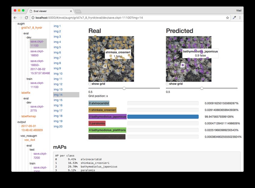
Figure 4: Example predictions on the crabs dataset. The grid is rendered in the middle row for
reference. Classes (species) are colour coded. For each image pair, ground truth on left and prediction
on right. Confidence threshold 0.5.

5.2   Evaluation on VOC12 dataset

Two models were trained on the VOC dataset, one using a 4x4 grid and one using a 7x7 grid. The
resulting mAPs on the dev test are 29.93% and 27.34%, respectively, which are below the state of the
art but the model parameters are not fine-tuned for this dataset. We focus mainly on small objects
that fit into a grid cell. The training was done with no data augmentation. Table 5 shows per-class
average precision (AP) scores and mAP results on train and dev sets.
Large objects that span across many grid cells are predicted more than once, but only considered
correct in the cell containing the centre of the ground truth label. This raises the level of false positives
at test time and can negatively influence training. For instance, if an object is in the middle between
two grid cells, both are equally qualified to make that prediction, but only one will contain the object
and during training this situation will be regarded as an error in the other grid cell.
Example predictions are shown in Figure 5

5.3   Evaluation on Steller Sea Lions Dataset

The aim of the NOAA Fisheries Kaggle competition is to predict population counts, not to detect
where objects are. The evaluation metric for the competition is mean column-wise root mean squared
error (RMSE). For N images and K classes, it is:
                                           v
                                       K u        N
                                   1  X    u1 X
                                           t        (yij − ŷij )2 ,                           (3)
                                   K i        N j

where the labels y and predictions ŷ are population counts.

                                                     8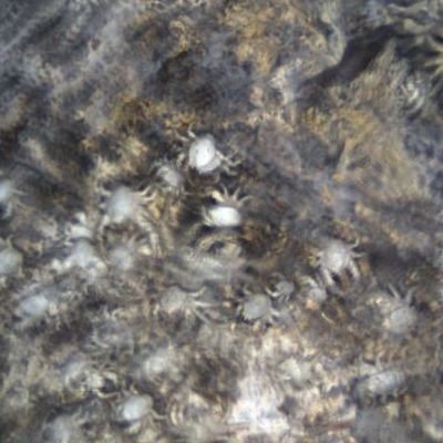
Table 5: Evaluation results on the VOC12 detection dataset. Class results are Average Precision (AP).
4x4 and 7x7 denote the grid size of our model configuration. Input images resized to 224x224 pixels.
No data augmentation was used and no fine-tuning of the model. Values in %.
                                   Train 7x7 Train 4x4 Dev 7x7 Dev 4x4
                    aeroplane      51.66       52.74        36.69       34.29
                    bicycle        55.19       52.00        22.46       23.37
                    bird           42.37       52.01        29.04       33.65
                    boat           45.87       50.67        24.00       27.47
                    bottle         51.56       46.62        14.79       14.38
                    bus            69.35       56.27        38.57       35.07
                    car            52.61       56.92        27.99       32.24
                    cat            47.69       61.27        31.56       38.95
                    chair          39.57       52.36        18.57       22.95
                    cow            57.38       56.83        25.57       31.30
                    diningtable 54.00          69.85        20.41       24.91
                    dog            51.58       62.07        31.08       35.35
                    horse          49.49       61.69        23.50       32.43
                    motorbike      55.91       58.58        29.69       28.17
                    person         54.09       65.14        40.60       47.76
                    pottedplant 40.74          49.22        18.11       21.33
                    sheep          55.27       60.86        35.92       36.32
                    sofa           52.88       65.97        16.83       20.28
                    train          47.68       47.79        30.18       32.39
                    tvmonitor      51.37       53.66        31.16       25.95
                    mAP            51.31       56.63        27.34       29.93

Figure 5: Example predictions on the VOC12 dataset. For each image pair, ground truth on left and
prediction on right. Confidence score shown next to object class name.

                                                 9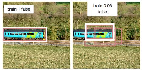
Table 6: Evaluation results on the Steller Sea Lions dataset. Class results are Average Precision (AP)
%. 4x4 and 7x7 denote the grid size of our model configuration. Dataset images sequentially sliced in
224x224 input images. mAP in %. RMSE is Mean Column-Wise RMSE at 0.5 confidence threshold.
                                      7x7 train 7x7 dev 4x4 train 4x4 dev
                  adult females         35.68       33.00       45.03        41.92
                  adult males           49.24       36.77       57.81        45.86
                  juveniles             39.91       31.87       47.52        38.86
                  pups                  36.38       32.36       43.27        37.98
                  subadult males        36.01       23.01       48.67        27.04
                  mAP                   39.44       31.40       48.46        38.33
                  RMSE                   1.69        1.68        1.49         1.52

We trained two models, grid 7x7 and grid 4x4. On the dev set we achieve 31.40% and 38.33%,
respectively. Training was done for 30 epochs. Mean Column-Wise RMSE at 0.5 confidence threshold
for 7x7 and 4x4 are 1.68 and 1.52, respectively. Note this is on the sliced dev set, not on the large
images from the original dataset. The values will likely be higher on the larger images. Results
illustrated in Table 6. At the time of writing, the top position in the competition leaderboard has
11.33729 RMSE on the official test set.

6       Implementation
The model was developed with TensorFlow (Abadi et al., 2015). I used parts of TensorBox3
(TensorFlow implementation of (Stewart et al., 2016)) as a reference point. My implementation is an
object detection network as opposed to only object localisation like TensorBox.
I implemented image and label readers for VOC, sea lions and crabs datasets along with tools used
for slicing images and labels. I implemented an evaluation, prediction and visualisation tool. The
predictions are stored in an sqlite databases and can be later used for visualisation and further analysis.
The visualisation tool allows viewing all trained models in a directory tree along with relevant
evaluation results on test, dev and training sets. The visualisation tool is a python (with flask) web
server and web page that shows evaluation metrics, class counts, images and predictions on the
images and precision-recall plots. A screenshot is shown in Figure 6.

References
Martín Abadi, Ashish Agarwal, Paul Barham, Eugene Brevdo, Zhifeng Chen, Craig Citro, Greg S.
 Corrado, Andy Davis, Jeffrey Dean, Matthieu Devin, Sanjay Ghemawat, Ian Goodfellow, Andrew
 Harp, Geoffrey Irving, Michael Isard, Yangqing Jia, Rafal Jozefowicz, Lukasz Kaiser, Manjunath
 Kudlur, Josh Levenberg, Dan Mané, Rajat Monga, Sherry Moore, Derek Murray, Chris Olah, Mike
 Schuster, Jonathon Shlens, Benoit Steiner, Ilya Sutskever, Kunal Talwar, Paul Tucker, Vincent
 Vanhoucke, Vijay Vasudevan, Fernanda Viégas, Oriol Vinyals, Pete Warden, Martin Wattenberg,
 Martin Wicke, Yuan Yu, and Xiaoqiang Zheng. TensorFlow: Large-scale machine learning
 on heterogeneous systems, 2015. URL http://tensorflow.org/. Software available from
 tensorflow.org.
M. Everingham, S. M. A. Eslami, L. Van Gool, C. K. I. Williams, J. Winn, and A. Zisserman. The
 pascal visual object classes challenge: A retrospective. International Journal of Computer Vision,
 111(1):98–136, January 2015.
Lowell W Fritz, Kathryn M Sweeney, Rodney G Towell, and Thomas Scott Gelatt. Aerial and
  Ship-based Surveys of Steller Sea Lions (Eumetopias Jubatus) Conducted in Alaska in June-July
  2013 Through 2015, and an Update on the Status and Trend of the Western Distinct Population
  Segment in Alaska. 2016.
Tsung-Yi Lin, Michael Maire, Serge Belongie, James Hays, Pietro Perona, Deva Ramanan, Piotr
  Dollár, and C Lawrence Zitnick. Microsoft coco: Common objects in context. In European
  Conference on Computer Vision, pp. 740–755. Springer, 2014.
    3
        https://github.com/TensorBox/TensorBox

                                                   10
Figure 6: Screenshot of the visualisation tool built to aid the development of this model. The
predictions seen in the page are all misclassified. Highlighting shows matching pair of ground truth
and prediction.
NOAA Fisheries. Noaa fisheries steller sea lion population count, 2017. URL https://www.
kaggle.com/c/noaa-fisheries-steller-sea-lion-population-count.
Joseph Redmon, Santosh Divvala, Ross Girshick, and Ali Farhadi. You only look once: Unified,
real-time object detection. In Proceedings of the IEEE Conference on Computer Vision and Pattern
Recognition, pp. 779–788, 2016.
Russell Stewart, Mykhaylo Andriluka, and Andrew Y Ng. End-to-end people detection in crowded
scenes. In Proceedings of the IEEE Conference on Computer Vision and Pattern Recognition, pp.
2325–2333, 2016.
Christian Szegedy, Wei Liu, Yangqing Jia, Pierre Sermanet, Scott Reed, Dragomir Anguelov, Du-
mitru Erhan, Vincent Vanhoucke, and Andrew Rabinovich. Going deeper with convolutions. In
Proceedings of the IEEE Conference on Computer Vision and Pattern Recognition, pp. 1–9, 2015.
Blair Thornton, Adrian Bodenmann, Oscar Pizarro, Stefan B Williams, Ariell Friedman, Ryota Naka-
jima, Ken Takai, Kaori Motoki, Tomo-o Watsuji, Hisako Hirayama, et al. Biometric assessment of
deep-sea vent megabenthic communities using multi-resolution 3d image reconstructions. Deep
Sea Research Part I: Oceanographic Research Papers, 116:200–219, 2016.
11You can also read