FILTER PRE-PRUNING FOR IMPROVED FINE-TUNING OF QUANTIZED DEEP NEURAL NETWORKS
←
→
Page content transcription
If your browser does not render page correctly, please read the page content below
Under review as a conference paper at ICLR 2021

F ILTER PRE - PRUNING FOR IMPROVED FINE - TUNING OF
QUANTIZED DEEP NEURAL NETWORKS

 Anonymous authors
 Paper under double-blind review

                                             A BSTRACT

         Deep Neural Networks(DNNs) have many parameters and activation data, and
         these both are expensive to implement. One method to reduce the size of the DNN
         is to quantize the pre-trained model by using a low-bit expression for weights
         and activations, using fine-tuning to recover the drop in accuracy. However, it is
         generally difficult to train neural networks which use low-bit expressions. One
         reason is that the weights in the middle layer of the DNN have a wide dynamic
         range and so when quantizing the wide dynamic range into a few bits, the step
         size becomes large, which leads to a large quantization error and finally a large
         degradation in accuracy. To solve this problem, this paper makes the following
         three contributions without using any additional learning parameters and hyper-
         parameters. First, we analyze how batch normalization, which causes the afore-
         mentioned problem, disturbs the fine-tuning of the quantized DNN. Second, based
         on these results, we propose a new pruning method called Pruning for Quantiza-
         tion (PfQ) which removes the filters that disturb the fine-tuning of the DNN while
         not affecting the inferred result as far as possible. Third, we propose a work-
         flow of fine-tuning for quantized DNNs using the proposed pruning method(PfQ).
         Experiments using well-known models and datasets confirmed that the proposed
         method achieves higher performance with a similar model size than conventional
         quantization methods including fine-tuning.

1   I NTRODUCTION

DNNs (Deep Neural Networks) greatly contribute to performance improvement in various tasks and
their implementation in edge devices is required. On the other hand, a typical DNN (He et al., 2015;
Simonyan & Zisserman, 2015) has the problem that the implementation cost is very large, and it is
difficult to operate it on an edge device with limited resources. One approach to this problem is to
reduce the implementation cost by quantizing the activations and weights in the DNN.
Quantizing a DNN using extremely low bits, such as 1 or 2 bits has been studied by
Courbariaux et al. (2015) and Gu et al. (2019). However, it is known that while such a bit re-
duction has been performed for a large model such as ResNet (He et al., 2015), it has not yet
been performed for a small model such as MobileNet (Howard et al., 2017; Sandler et al., 2018;
Howard et al., 2019), and is very difficult to apply to this case. For models that are difficult to quan-
tize, special processing for the DNN is required before quantization. On the other hand, although
fine-tuning is essential for quantization with extremely low bit representation, few studies have been
conducted on pre-processing for easy fine-tuning of quantized DNNs. In particular, it has been ex-
perimentally shown from previous works (Lan et al., 2019; Frankle & Carbin, 2018) that, regardless
of quantization, some weights are unnecessary for learning or in fact disturb the learning process.
Therefore, we focused on the possibility of the existence of weights that specially disturb the fine-
tuning quantized DNN and to improve the performance of the quantized DNN after fine-tuning by
removing those weights.

                                                   1
Under review as a conference paper at ICLR 2021

Figure 1: This is a diagram of the proposed pruning method PfQ. As mentioned in subsection 3.1,
the filters with a very small running variance can approximate its output by βi . At this time, by
pruning the filters and correcting the bias of the next convolution using βi as described above, the
DNN can be pruned without affecting the output as far as possible.

2     R ELATED WORK AND P ROBLEM
2.1   C ONVENTIONAL Q UANTIZATION WORKS

In order to reduce the implementation cost of DNN in hardware, many methods of reduction by
pruning (Molchanov et al., 2019; You et al., 2019; He et al., 2019) and quantization (Gu et al., 2019;
Gong et al., 2020; Fan et al., 2020; Uhlich et al., 2019; Sheng et al., 2018; Nagel et al., 2019) have
been studied. Research is also underway in network architectures such as depthwise convolu-
tion and pointwise convolution (Howard et al., 2017), which are arithmetic modules that maintain
high performance even when both the number of operations and the model capacity are kept small
(Howard et al., 2017; Sandler et al., 2018; Howard et al., 2019). Knowledge Transfer (Hinton et al.,
2015; Zagoruyko & Komodakis, 2016; Radosavovic et al., 2018; Chen et al., 2019) is also being
studied as a special learning method for achieving high performance in these compression technolo-
gies and compressed architectures.
There have been various approaches to studies in DNN compression using quantization. DNN quan-
tization is usually done for activations and weights in DNN. As a basic approach to quantization,
there are some methods for a pre-trained model of which one uses only quantization (Sheng et al.,
2018; Nagel et al., 2019) and another uses fine-tuning (Gong et al., 2019; Gu et al., 2019; Jung et al.,
2019; Uhlich et al., 2019; Gong et al., 2020; Fan et al., 2020). Cardinaux et al. (2020) and Han et al.
(2015) propose a method for expressing values that are as precise as possible. However, the sim-
plest expression method is easier to calculate and implement in hardware, so expressions to divide
the range of quantized values by a linear value (Jacob et al., 2018; Sheng et al., 2018; Nagel et al.,
2019; Gu et al., 2019; Gong et al., 2019; 2020; Jung et al., 2019) or a power of 2 value (Lee et al.,
2017; Li et al., 2019) are widely used at present in quantization research.
It is known that fine-tuning is essential to quantize DNN with low bits in order not to decrease accu-
racy as much as possible. Jacob et al. (2018) shows that an accuracy improvement can be expected
by fine-tuning with quantization. Since the quantization function is usually non-differentiable, the
gradient in the quantization function is often approximated by STE (Bengio et al., 2013). However,
in the case of quantization with low bits, the error is very large in the approximation by STE, and it
is known that it is difficult to accurately propagate the gradient backward from the output side to the
input side, making learning difficult. In order to solve this problem, Gong et al. (2019), Fan et al.
(2020) and Darabi et al. (2018) proposed the backward quantization function so that the gradient can
be propagated to the input side as accurately as possible. Gu et al. (2019) and Banner et al. (2018)
considered activations and weights in DNN as random variables, and proposed an approach to op-
timize the stochastic model behind DNN so that activations and weights in DNN become vectors
which are easy to quantize. Jung et al. (2019) and Uhlich et al. (2019) considered that it is important

                                                   2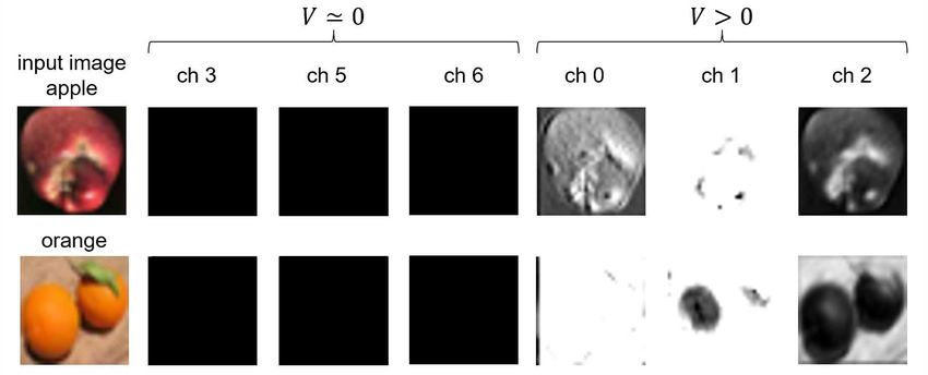
Under review as a conference paper at ICLR 2021

for performance to determine the dynamic range of vectors to be quantized appropriately, and it is
proposed that this dynamic range is also learned as a learning parameter.

2.2      P ROBLEM OF WIDE DYNAMIC RANGE ON QUANTIZATION

It is important to set the dynamic range appropriately in the quantization. In modern network ar-
chitectures, most of the computation is made up of a block of convolution and batch normalization
(BN). It is known that the above block can be replaced by the equivalent convolution, and quanti-
zation is performed after this replacement. Thus, it is possible to suppress the quantization error
rather than quantizing the convolution and BN separately. On the other hand, it is also known that
the dynamic range of the convolution may be increased by this replacement (Sheng et al., 2018;
Nagel et al., 2019). In order to explain this in detail, the calculation formulas of convolution and BN
in pre-training are described. First, the equation for convolution is described as follows
                                   XX
                        C(o,j,k) =           w(o,i,u,v) x(i,j+u,k+v) + b(o) ,                        (1)
                                          i       (u,v)

where C(o,j,k) is the o-th convolution output feature at the coordinate (j, k), w(o,i,u,v) is the weight
of the kernel coordinates (u, v) in the i-th input map, and x(i,j+u,k+v) is the input data. For sim-
plicity, C(o,j,k) is represented as vector C(o) = (c(o,1) , ..., c(o,N ) )1 and w(o,i,u,v) is represented as
vector w(o,i) if it is not necessary. Next, the calculation formula for BN is described as
                                          C(o) − µ(o)
                                   B(o) = p              γ(o) + β(o) ,                                  (2)
                                            (σ(o) )2 + ǫ
where B(o) is the o-th BN output feature2 . µ(o) , (σ(o) )2 are respectively calculated by equation (3),
(4) during the training or by equation (7), (8) during the inference. γ(o) , β(o) are respectively the
scaling factor and shift amounts of BN. The mean and variance are calculated as
                                                            N
                                                          1 X
                                         µ(o)       =         c(o,n)                                    (3)
                                                          N n
                                                            N
                                              2           1 X              2
                                    (σ(o) )         =         c(o,n) − µ(o) .                           (4)
                                                          N n
At the time of inference or the fine-tuning of quantization for the pre-trained model, BN can be
folded into convolution by inserting equation (1) into (2). The new weight (ŵ(o,i,u,v) ) and bias
(b̂(o) ) of the convolution when BN is folded in the convolution are calculated by
                                        γ(o)
                        ŵ(o,i) = q             w(o,i)                                         (5)
                                         (τ )
                                      V(o) + ǫ
                                        γ(o)                      γ(o)       (τ )
                          b̂(o) = q             b(o) + β(o) − q           M(o) ,               (6)
                                         (τ )                      (τ )
                                      V(o) + ǫ                   V(o) + ǫ
            (τ )   (τ )
where M(o) , V(o) are respectively the mean (running mean) and variance (running variance) of BN
used at inference, and the values are calculated as
                                  (τ )                (τ −1)
                               M(o)      =         M(o)        ρ + µ(o) (1 − ρ)                         (7)
                                  (τ )               (τ −1)        N
                                V(o)     =         V(o)       ρ + (σ(o) )2 (1 − ρ)
                                                                        ,                        (8)
                                                                 N −1
where τ is an iteration index, and is omitted in this paper when not specifically needed, and ρ is a
hyper-parameter of BN in pre-training so that 0 < ρ < 1. The initial values of (7) and (8) are set
before learning in the same way as weights such as convolution.
Sheng et al. (2018) pointed out that the dynamic range of the weights of depthwise convolution is
   1
       N is the number of elements in a channel C(o) .
   2
       Vector and scalar operations are performed by implicitly broadcasting scalars.

                                                                 3
Under review as a conference paper at ICLR 2021
large, which leads to the large quantization error. They also pointed out the relationship that the
filters (sets of weights) with wide dynamic range correspond to the running variances of the BN
with small magnitude. Nagel et al. (2019) attacked this problem by adjusting scales of weights of
consecutive depthwise and pointwise convolutions without affecting the outputs of the pointwise
convolution. However, they cannot solve the problem in quantization completely.
In this study, we theoretically analyze the weights with the running variances which have small
magnitude and show that certain weights disturb the fine-tuning of the quantized DNN. Based on
this analysis, we propose a new quantization training method which can solve the problem and
improve the performance (section 4).
3 P ROPOSAL
3.1 W EIGHTS D ISTURBING L EARNING
We analyze how the fine-tuning is affected when the following condition holds
(L,τ )
V(c) ≃ 0, (9)
(L,τ )
where V(c) is the running variance (8) of cth-channel in Lth-BN. When (9) holds regarding a
significantly large τ , the term of the left side and the first term of the right side in (8) are close to
zero. Therefore, it is necessary that the second term of the right side in (8) close to zero to hold (8).
As the result, the variance (σ(c) )2 ≃ 0 holds, the following equation
(L) (L)
|C(c,n) − µ(c) | ≃ 0 (10)
holds for arbitrary n ∈ {1, ..., N } and input data from (4). ǫ in (2) is usually set to satisfy ǫ ≫ 0.
Therefore, in the case of (σ(c) )2 ≃ 0, since (σ(c) )2 ≪ ǫ holds, the following equation
(L) (L)
B(c) ≃ β(c) (11)
holds from (2) and (10). Since the output of BN is a constant value by (11) regardless of the input
data, the following convolution can be calculated as
(L+1)
X X (L+1) (L+1) X (L+1) (L) (L+1)
C(o,j,k) ≃ w(o,i,u,v) x(i,j+u,k+v) + w(o,c,u,v) Act(β(c) ) + b(o) (12)
i (u,v) (u,v)
i6=c
(L+1) (L+1) (L+1)
XX
= w(o,i,u,v) x(i,j+u,k+v) + b̂(o) (13)
i (u,v)
i6=c
(L+1) (L+1) (L+1) (L)
b̂(o) = b(o) + U (w(o,c) , β(c) ) (14)
(L+1) (L)
X (L+1) (L)
U (w(o,c) , β(c) ) = w(o,c,u,v) Act(β(c) ) (15)
(u,v)
where Act(∗) is the activation function. This is equivalent to the bias of the L + 1-th convolution
being (14). The bias of (14) is updated as
(L+1,τ ) (L+1,τ −1) (L+1,τ −1) (L,τ −1)
b̂(o) = b(o) + U (w(o,c) , β(c) )
(L+1,τ −1) (L+1,τ −1) (L,τ −1)
+ ∆b(o) + ∆U (w(o,c) , β(c) ) (16)
where τ is an index of the iteration to express the bias before and after the update. At the step of
quantization, since each of the first and second terms of (14) is quantized, the quantization error tends
to be larger than when the whole of (14) is quantized. Further, in addition to the quantization error
of (14), equation (16) adds an approximation error in approximating the gradient of the quantization
function to the third and fourth terms, respectively. Therefore, it can be seen that the quantization
(L+1)
error of b̂(o) tends to be larger than that of the other weights in the fine-tuning of the quantized
DNN. From the above, it can be seen that the filters satisfying (9) disturb the fine-tuning.
4Under review as a conference paper at ICLR 2021
3.2 P ROPOSAL OF N EW P RUNING M ETHOD TO R EMOVE W EIGHTS D ISTURBING T RAINING
(τ )
As mentioned in subsection 3.1, weights that satisfy V(o) ≃ 0 extend the dynamic range and disturb
the fine-tuning of the quantized DNN. Therefore, we propose a new pruning method, illustrated in
Figure 1, called Pruning for Quantization (PfQ), that solves the described problem by removing the
weights that satisfies the following conditional
(L,τ )
V(o)Under review as a conference paper at ICLR 2021
Algorithm 1 Proposal of Quantization Workflow
Input: pre-trained model, dataset, training hyperparameters (bitwidth, epochs eA , eW , the other
training parameters)
Output: quantized model
1: Perform PfQ operation to the pre-trained model
2: for i = 0 to eA do
3: Fine-tune the pre-trained model for quantized activations
4: end for
5: Perform PfQ operation to the fine-tuned model for the quantized activations
6: Fold BN
7: for i = 0 to eW do
8: Fine-tune the model for the quantized activations and weights
9: end for
10: return quantized model
4.1 E XPERIMENTAL S ETTINGS
We experiment with the classification task using CIFAR-100 and imagenet1000 as datasets. The
learning rate was calculated by the following equation
l−1 × 1 + cos e − w π
(e ≧ w)
le = λ (19)
l−1 × e
(e < w),
w
where e is the number of epochs, l−1 is the initial learning rate, w is the number of warm-up
epochs, and λ is the period of the cosine curve. The learning rate was reduced by a cosine curve
(Loshchilov & Hutter, 2016) during e ≧ w. In the following experiments, the proposed method
learned 100 epochs in the each fine-tuning in Algorithm 1, respectively. We used DSQ (Gong et al.,
2019), PACT (Choi et al., 2018; Wang et al., 2018) and DFQ (Nagel et al., 2019) as quantization
methods to compare with our proposed method. The performance of DSQ and PACT are directly
referenced from the values in the paper, but regarding DFQ, the performance of the fine-tuning of
the quantized DNN was not described in the paper. Therefore the performance of DFQ was obtained
by our own experiment with 200 epochs fine-tuning.
In this paper, we use the quantization function given by the following
min(max(x, m), M ) − m
Q(x) = round × scale + m (20)
scale
M −m
scale = (21)
2n
where x represents the input data (an activation or a weight) of the quantization function, n repre-
sents the bit width, and m, M represent the lower limit and upper limit of the quantization range, re-
spectively. We use STE to calculate the gradient. In this paper, we use MobileNetV1 (Howard et al.,
2017) and MobileNetV2 (Sandler et al., 2018) as the network architectures. At the time of quanti-
zation, for quantization of activations, all activations except the last layer and addition layers (i.e.
outputs of skip connection) were quantized, and for weights, all convolutions, depthwise convolu-
tions and affines including the first and last layers were quantized.
In this study, ǫ = 0.00001 was used as ǫ in (17). This is the default value of the BN in NNabla
(Sony).
4.2 A BLATION S TUDY
4.2.1 E FFECT OF D ISTURBING W EIGHTS
In this section, we made a comparative experiment to confirm that PfQ eliminates the bad effect on
the fine-tuning of the quantized DNN described in subsection 3.1. In addition, in order to confirm
the effect of the bias correction in PfQ, we made the experiment even in the case where the bias
6Under review as a conference paper at ICLR 2021
correction was excluded. We made experiments for MobileNetV1 and MobileNetV2 for the clas-
sification task of CIFAR-100. In the experiment of CIFAR-100 in this paper, the GPU was single
(2080Ti) and the batch size was 16. We made the pre-trained models of the two network architec-
tures by the following experiment: the number of epochs was 600, the optimizer was momentum
SGD, the moment was 0.9, the learning rate settings in (19) were l−1 = 0.16, w = 0, λ = 40, and
the learning rate decay was not used. In the fine-tuning of the quantized DNN the following settings
were used: the number of epochs was 100, the optimizer was the same as the pre trained model, the
learning rate settings in (19) were l−1 = 0.001, w = 0, λ = 100, and the weight decay was 0.0001.
Table 1: Top1 Accuracy comparison between pruned and no pruned models
PfQ
Model Activation bitwidth Evaluation original PfQ
(w/o bias correction)
Accuracy 76.34 76.67 76.75
MobileNetV1 4
MAC 510M 367M 367M
Accuracy 74.17 75.14 75.26
MobileNetV1 3
MAC 510M 367M 367M
Accuracy 74.04 74.67 75.00
MobileNetV2 4
MAC 147M 93M 93M
Accuracy 71.36 72.17 72.28
MobileNetV2 3
MAC 147M 93M 93M
The experimental results are summarized in Table 1. Regarding the accuracy in Table 1, Table 1
shows that the fine-tuning after using PfQ gives better performance in all experiments, and it can be
solved that the bad effect on the fine-tuning of the quantized DNN described in 3.1. In particular,
in PfQ (w/o bias correction), the accuracy is higher than that of the original, and the difference is
larger for 3 bits than 4 bits, indicating that the influence of the quantization error (i.e. the 4th term in
(16)) in the backward calculation is large. MobileNetV1 and MobileNetV2 in the columns of PfQ
in Table 1 are pruned with the weights by 31.86% and 35.74%, respectively. Thus, the number of
MACs is also reduced.
4.2.2 S OLVING DYNAMIC R ANGE P ROBLEM
In this section, we confirmed that PfQ can suppress the increase in the dynamic range of the weights
after folding BN. The models that we used are MobileNetV1 and MobileNetV2 used in Table 1.
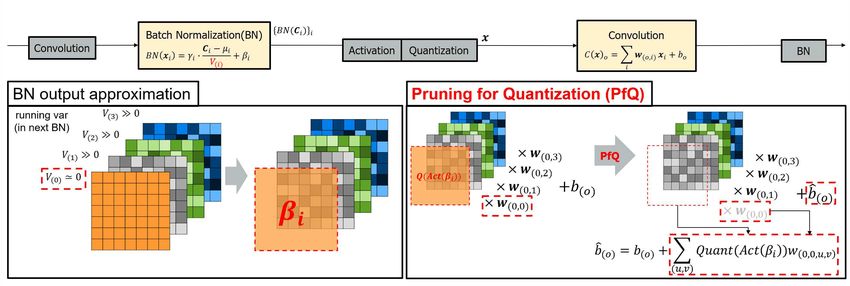
Figure 2: This is a figure comparing the dynamic range of the weights after folding BN with re-
spect to using or not using PfQ. The left figure is about MobileNetV1 and the right one is about
MobileNetV2. The blue bin is not using PfQ and the red one is using PfQ. The vertical axis is the
dynamic range value (i.e. weight max - weight min), and the horizontal axis is the layer. In each
figure of MobileNetV1 and MobileNetV2, the left side on the horizontal axis is the layer on the
input side.
From the results in Figure 2, it can be seen that PfQ improves the wide dynamic range.
7Under review as a conference paper at ICLR 2021
4.2.3 E FFECT OF P ROPOSED Q UANTIZATION W ORKFLOW
In this section, we confirm the effect of Algorithm 1. Table 2 shows the results of comparing the
performance between quantization using Algorithm 1 and the fine-tuning of the DNN with activa-
tions and weights quantization simultaneously once after performing PfQ. The experiments are the
classification task of CIFAR-100 using MobileNetV1 and MobileNetV2. In the each fine-tuning in
Algorithm 1, the number of epochs was 100, the optimizer was momentum SGD, the moment was
0.9, the learning rate settings in (19) were w = 0, λ = 100. Regarding the fine-tuning once with
PfQ, the number of epochs is 200 in order to be the same number of the total epochs in Algorithm
1.
Table 2: Effect of proposed quantization workflow
Bitwidth fine-tune once
Model Evaluation Algorithm 1
(Activation/Weight) (w/ PfQ)
Accuracy 74.69 75.31
MobileNetV1 A4/W4
MAC 367M 367M
Accuracy 71.56 70.85
MobileNetV1 A3/W3
MAC 367M 367M
Accuracy 72.78 72.7
MobileNetV2 A4/W4
MAC 93M 92.4M
Accuracy 66.29 68.96
MobileNetV2 A3W3
MAC 93M 93M
Table 2 shows that Algorithm 1 is better. Although the performance of Algorithm 1 is lower than
that of the fine-tuning once with PfQ for A3W3 of MobileNetV1 and A4W4 of MobileNetV2, the
difference is small, and Algorithm 1 which can often reduce the MAC is considered to be better.
4.3 C OMPARISON TO OTHER METHODS
In this section, we apply the proposed quantization workflow using PfQ to the pre-trained model.
Here, we compare the performance of the proposed method with that of the other quantization
methods. The experimental settings common to each are described below. We used MobileNetV1
and MobileNetV2 as a network architecture. In the each fine-tuning in Algorithm 1, the number of
epochs was 100, the optimizer was momentum SGD, the moment was 0.9, the learning rate settings
in (19) were w = 0, λ = 100. In the experiment of DFQ, the number of epochs was 200, the learning
rate settings in (19) were w = 0, λ = 200. The optimizer, the batch size, the initial learning rate l−1
and the weight decay settings were the same settings as Table 3 and Table 4.
4.3.1 CIFAR-100 CLASSIFICATION EXPERIMENT
In this subsection, we compare the performance of the proposed quantization method with DFQ us-
ing fine-tuning in the classification task of CIFAR-100. Next, we explain the experimental settings.
We used a single GPU (2080Ti) for the learning in CIFAR-100. The same pre-trained model as
subsection 4.2.1 was used. In our method, we used the same settings as subsection 4.2.1 in the first
fine-tuning for quantized activations only in Algorithm 1. In the settings of the second fine-tuning
for quantized activations and weights in the Algorithm 1, the optimizer was SGD (i.e. the moment
was 0), l−1 = 0.0005, the weight decay was 0.00001. In the settings of DFQ, the optimizer was
SGD, l−1 = 0.001, and the weight decay was 0.0001.
The experimental results are summarized in Table 3, which shows that the performance of the pro-
posed method is better than DFQ with fine-tuning. Also, 2 PfQ operations in the proposed quan-
tization workflow pruned the weights by 36.17% and 34.36% in the A4/W4 and A3/W3 models,
respectively. Thus, the number of MACs was also reduced.
4.3.2 IMAGENET 1000 CLASSIFICATION EXPERIMENT
In this subsection, we compare the performance of the proposed quantization method with the other
quantization method in the classification task of imagenet1000. The methods used for comparison
are DSQ and PACT which achieve high performance with 4 bits in the activations and weights
8Under review as a conference paper at ICLR 2021
Table 3: Top1 Accuracy comparison CIFAR-100
Bitwidth DFQ
Model Evaluation Ours
(Activation/Weight) (w/ fine-tune)
Accuracy 71.57 75.31
MobileNetV1 A4/W4
MAC 510M 367M
Accuracy 61.58 70.85
MobileNetV1 A3/W3
MAC 510M 367M
Accuracy 72.14 72.7
MobileNetV2 A4/W4
MAC 147.2M 92.4M
Accuracy 68.05 68.96
MobileNetV2 A3/W3
MAC 147.2M 93.0M
for MobileNetV2, and DFQ. Next, the experimental settings are described. The experiment of the
imagenet1000 was learned using 4 GPUs (tesla v100 x4), the optimizer was momentum SGD, the
moment was 0.9, and the weight decay was 0.00001. The pre-trained model was learned by the
following settings. The number of epochs was 120, the batch size was 256, the learning rate settings
in (19) were l−1 = 0.256, w = 16, λ = 104. The settings for the fine-tuning of the quantized
DNN are described below. In our method, in addition to the above settings, the batch size was 64,
and the initial learning rate was l−1 = 0.01 in the first fine-tuning for quantized activations only in
Algorithm 1. In the second fine-tuning for quantized activations and weights in the Algorithm 1, the
initial learning rate was l−1 = 0.0001. In the experimental settings of DFQ, the batch size was 128,
the initial learning rate was l−1 = 0.0001.
Table 4: Top1 Accuracy comparison imagenet1000
Bitwidth DFQ
Evaluation PACT DSQ Ours
(Activation/Weight) (w/ fine-tune)
Accuracy 57.44 61.39 64.8 67.48
A4/W4
MAC 313M 313M 313M 261M
The experimental results are summarized in Table 4, which shows that the quantization performance
of the proposed method is the best compared to the other quantization methods. In our approach,
2 PfQ operations in the proposed quantization workflow pruned the weights by 10.29%. Thus, the
number of MACs was also reduced.
These results show that PfQ and the proposed quantization workflow make it easy to fine-tune the
quantized DNN and can make high-performance models even with low bits. On the other hand, in
this method, STE is used as the gradient of the quantization function, and the problem of degradation
of the gradient due to quantization, which is often raised as a problem in the study of quantization, is
not addressed. Therefore, further performance improvement can be expected if a technique to cope
with gradient degradation during the fine-tuning of the quantized DNN such as DSQ is used together
with the proposal of this paper.
5 C ONCLUSION
In this paper, we propose PfQ to solve the dynamic range problem in the fine-tuning of the quantized
DNN and the problem that the quantization errors tend to accumulate in some bias, and we propose
a new quantization workflow including PfQ. Since PfQ is a type of filter pruning, it also has the
effect of reducing the number of weights and the computational costs. Moreover, our method is
very easy to use because there are no additional hyper-parameters and learning parameters like the
conventional pruning and quantization methods.
R EFERENCES
Ron Banner, Yury Nahshan, Elad Hoffer, and Daniel Soudry. ACIQ: analytical clip-
ping for integer quantization of neural networks. CoRR, abs/1810.05723, 2018. URL
9Under review as a conference paper at ICLR 2021
http://arxiv.org/abs/1810.05723.
Yoshua Bengio, Nicholas Léonard, and Aaron Courville. Estimating or propagating gradients
through stochastic neurons for conditional computation. arXiv preprint arXiv:1308.3432, 2013.
Fabien Cardinaux, Stefan Uhlich, Kazuki Yoshiyama, Javier Alonso Garcı́a, Lukas Mauch, Stephen
Tiedemann, Thomas Kemp, and Akira Nakamura. Iteratively training look-up tables for network
quantization. IEEE Journal of Selected Topics in Signal Processing, 14(4):860–870, 2020.
Hanting Chen, Yunhe Wang, Chang Xu, Zhaohui Yang, Chuanjian Liu, Boxin Shi, Chunjing Xu,
Chao Xu, and Qi Tian. Data-free learning of student networks. In Proceedings of the IEEE
International Conference on Computer Vision, pp. 3514–3522, 2019.
Jungwook Choi, Zhuo Wang, Swagath Venkataramani, Pierce I-Jen Chuang, Vijayalakshmi Srini-
vasan, and Kailash Gopalakrishnan. PACT: parameterized clipping activation for quantized neural
networks. CoRR, abs/1805.06085, 2018. URL http://arxiv.org/abs/1805.06085.
Matthieu Courbariaux, Yoshua Bengio, and Jean-Pierre David. Binaryconnect: Training deep neural
networks with binary weights during propagations. In Advances in neural information processing
systems, pp. 3123–3131, 2015.
Sajad Darabi, Mouloud Belbahri, Matthieu Courbariaux, and Vahid Partovi Nia.
BNN+: improved binary network training. CoRR, abs/1812.11800, 2018. URL
http://arxiv.org/abs/1812.11800.
Angela Fan, Pierre Stock, Benjamin Graham, Edouard Grave, Rémi Gribonval, Hervé Jégou,
and Armand Joulin. Training with quantization noise for extreme model compression. ArXiv,
abs/2004.07320, 2020.
Jonathan Frankle and Michael Carbin. The lottery ticket hypothesis: Training pruned neural net-
works. CoRR, abs/1803.03635, 2018. URL http://arxiv.org/abs/1803.03635.
Cheng Gong, Yao Chen, Ye Lu, Tao Li, Cong Hao, and Deming Chen. Vecq: Minimal loss dnn
model compression with vectorized weight quantization. IEEE Transactions on Computers, 2020.
Ruihao Gong, Xianglong Liu, Shenghu Jiang, Tianxiang Li, Peng Hu, Jiazhen Lin, Fengwei Yu, and
Junjie Yan. Differentiable soft quantization: Bridging full-precision and low-bit neural networks.
In Proceedings of the IEEE International Conference on Computer Vision, pp. 4852–4861, 2019.
Jiaxin Gu, Junhe Zhao, Xiaolong Jiang, Baochang Zhang, Jianzhuang Liu, Guodong Guo, and Ron-
grong Ji. Bayesian optimized 1-bit cnns. In Proceedings of the IEEE International Conference
on Computer Vision, pp. 4909–4917, 2019.
Song Han, Huizi Mao, William J Dally, et al. Deep compression: Compressing deep neural networks
with pruning. trained quantization and huffman coding, 56(4):3–7, 2015.
Kaiming He, Xiangyu Zhang, Shaoqing Ren, and Jian Sun. Deep residual learning for image recog-
nition. CoRR, abs/1512.03385, 2015. URL http://arxiv.org/abs/1512.03385.
Yang He, Ping Liu, Ziwei Wang, Zhilan Hu, and Yi Yang. Filter pruning via geometric median
for deep convolutional neural networks acceleration. In Proceedings of the IEEE Conference on
Computer Vision and Pattern Recognition, pp. 4340–4349, 2019.
Geoffrey Hinton, Oriol Vinyals, and Jeff Dean. Distilling the knowledge in a neural network. arXiv
preprint arXiv:1503.02531, 2015.
Andrew Howard, Mark Sandler, Grace Chu, Liang-Chieh Chen, Bo Chen, Mingxing
Tan, Weijun Wang, Yukun Zhu, Ruoming Pang, Vijay Vasudevan, Quoc V. Le, and
Hartwig Adam. Searching for mobilenetv3. CoRR, abs/1905.02244, 2019. URL
http://arxiv.org/abs/1905.02244.
Andrew G. Howard, Menglong Zhu, Bo Chen, Dmitry Kalenichenko, Weijun Wang, To-
bias Weyand, Marco Andreetto, and Hartwig Adam. Mobilenets: Efficient convolutional
neural networks for mobile vision applications. CoRR, abs/1704.04861, 2017. URL
http://arxiv.org/abs/1704.04861.
10Under review as a conference paper at ICLR 2021
Benoit Jacob, Skirmantas Kligys, Bo Chen, Menglong Zhu, Matthew Tang, Andrew Howard,
Hartwig Adam, and Dmitry Kalenichenko. Quantization and training of neural networks for
efficient integer-arithmetic-only inference. In Proceedings of the IEEE Conference on Computer
Vision and Pattern Recognition, pp. 2704–2713, 2018.
Sangil Jung, Changyong Son, Seohyung Lee, Jinwoo Son, Jae-Joon Han, Youngjun Kwak, Sung Ju
Hwang, and Changkyu Choi. Learning to quantize deep networks by optimizing quantization
intervals with task loss. In Proceedings of the IEEE Conference on Computer Vision and Pattern
Recognition, pp. 4350–4359, 2019.
Janice Lan, Rosanne Liu, Hattie Zhou, and Jason Yosinski. Lca: Loss change allocation for neural
network training. In Advances in Neural Information Processing Systems, pp. 3619–3629, 2019.
Edward H Lee, Daisuke Miyashita, Elaina Chai, Boris Murmann, and S Simon Wong. Lognet:
Energy-efficient neural networks using logarithmic computation. In 2017 IEEE International
Conference on Acoustics, Speech and Signal Processing (ICASSP), pp. 5900–5904. IEEE, 2017.
Yuhang Li, Xin Dong, and Wei Wang. Additive powers-of-two quantization: An efficient non-
uniform discretization for neural networks. In International Conference on Learning Representa-
tions, 2019.
Ilya Loshchilov and Frank Hutter. SGDR: stochastic gradient descent with restarts. CoRR,
abs/1608.03983, 2016. URL http://arxiv.org/abs/1608.03983.
Pavlo Molchanov, Arun Mallya, Stephen Tyree, Iuri Frosio, and Jan Kautz. Importance estimation
for neural network pruning. In Proceedings of the IEEE Conference on Computer Vision and
Pattern Recognition, pp. 11264–11272, 2019.
Markus Nagel, Mart van Baalen, Tijmen Blankevoort, and Max Welling. Data-free quantiza-
tion through weight equalization and bias correction. CoRR, abs/1906.04721, 2019. URL
http://arxiv.org/abs/1906.04721.
Ilija Radosavovic, Piotr Dollár, Ross Girshick, Georgia Gkioxari, and Kaiming He. Data distillation:
Towards omni-supervised learning. In Proceedings of the IEEE conference on computer vision
and pattern recognition, pp. 4119–4128, 2018.
Mark Sandler, Andrew G. Howard, Menglong Zhu, Andrey Zhmoginov, and Liang-Chieh Chen.
Inverted residuals and linear bottlenecks: Mobile networks for classification, detection and seg-
mentation. CoRR, abs/1801.04381, 2018. URL http://arxiv.org/abs/1801.04381.
Tao Sheng, Chen Feng, Shaojie Zhuo, Xiaopeng Zhang, Liang Shen, and Mickey Aleksic. A
quantization-friendly separable convolution for mobilenets. CoRR, abs/1803.08607, 2018. URL
http://arxiv.org/abs/1803.08607.
Karen Simonyan and Andrew Zisserman. Very deep convolutional networks for large-scale image
recognition. In International Conference on Learning Representations, 2015.
Sony. Neural network libraries (nnabla). https://github.com/sony/nnabla.
Stefan Uhlich, Lukas Mauch, Fabien Cardinaux, Kazuki Yoshiyama, Javier Alonso Garcia, Stephen
Tiedemann, Thomas Kemp, and Akira Nakamura. Mixed precision dnns: All you need is a good
parametrization. arXiv preprint arXiv:1905.11452, 2019.
Kuan Wang, Zhijian Liu, Yujun Lin, Ji Lin, and Song Han. HAQ: hardware-aware automated quan-
tization. CoRR, abs/1811.08886, 2018. URL http://arxiv.org/abs/1811.08886.
Zhonghui You, Kun Yan, Jinmian Ye, Meng Ma, and Ping Wang. Gate decorator: Global filter
pruning method for accelerating deep convolutional neural networks. In Advances in Neural
Information Processing Systems, pp. 2133–2144, 2019.
Sergey Zagoruyko and Nikos Komodakis. Paying more attention to attention: Improving the perfor-
mance of convolutional neural networks via attention transfer. arXiv preprint arXiv:1612.03928,
2016.
11Under review as a conference paper at ICLR 2021
A A PPENDIX
A.1 E XPERIMENTS U SING VALIDATION SET
Algorithm 1 needs the fixed number of epochs in the experiments. So we made the experiments not
using the fixed number of epochs and using the value of accuracy drop. The accuracy check during
the training used validation set apart from training set and test set. We split a separate validation
set out of the original training set by randomly sampling 50 images from the training set for each
category. We set the accuracy drop 0.5% in the each fine-tuning in Algorithm 1 and 1.0% in DFQ.
Then the end numbers of epochs were 82 and 80 during the each fine-tuning in Algorithm 1 and the
end number of epoch of DFQ was 200 that was we set max epochs. The result is Table 5.
Table 5: Using Accuracy Drop
Bitwidth
Model Evaluation DFQ Ours
(Activation/Weight)
Accuracy 70.00 71.58
MobileNetV2 A4/W4
MAC 147.2M 92.4M
A.2 V ISUALIZE L OW VARIANCE C HANNELS
We claimed in subsection 3.1 that the outputs of some channels whose running variance close to
zero are the constant values. In this subsection, we confirmed the fact and the result was Figure 3.
Figure 3 shows that the channels whose running variances are close to zero are the constant value.
The model we used in Figure 3 was the pre-trained model in subsection 4.2.1. The input images are
in the CIFAR-100 training set.
Figure 3: This is the visualized channels of the first BN outputs after the first convolution in Mo-
bileNetV2. The input images are apple and orange, respectively. The running variance of the channel
3,5,6 are close to zero and that of the channel 0,1,2 are not close to zero.
12You can also read