Identifying nuclei in divergent images: Data Science Bowl 2018 - Udacity, Machine Learning Nanodegree Christopher Marks August 31st, 2018

Identifying nuclei in divergent images:
       Data Science Bowl 2018

    Udacity, Machine Learning Nanodegree

             Christopher Marks

             August 31st, 2018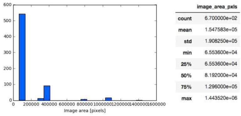

Table of Contents

Table of Contents                     2

I. Definition                         3
   Project Overview                   3
   Problem Statement                  4
   Metrics                            5

II. Analysis                          5
   Data Exploration                   5
   Exploratory Visualization          6
   Algorithms and Techniques          7
   Benchmark                          8

III. Methodology                      8
   Data Preprocessing                 8
   Implementation                     8
   Refinement                        10

IV. Results                          11
   Model Evaluation and Validation   11
   Justification                     12

V. Conclusion                        13
   Free-Form Visualization           13
   Reflection                        13
   Improvement                       14

References                           15

I. Definition

Project Overview
In the biomedical sciences, the process of nucleus detection is typically performed by individual
researchers manually going through scans. Automating this process using deep learning
techniques has the potential to speed up the process of finding cures for diseases ranging from
Alzheimer’s to cancer. A recent competition on Kaggle1 asks participants to construct a model
that can accurately identify the nuclei in images of cells. This capstone project will focus on
constructing an effective model for this challenge.

There’s a number of research projects that have applied these techniques already. Litjens et. al
(2017) provide a survey on the use of deep learning techniques in medical image analysis,
summarising over 300 contributions to this field. A specific example of this kind of research is
Sirinukunwattana et. al (2016), who use a spatially constrained convolutional neural network
(CNN) to detect and classify nuclei in a dataset of 20,000 annotated colon cancer images. The
benefit of this architecture is that it doesn’t require segmentation of the nuclei, and they find that
their chosen architecture produces the highest F1 score compared to other published
approaches. Sornapudi et. al (2018) find similar success applying a CNN architecture to a nuclei
segmentation problem on a dataset of 133 histology images, achieving an accuracy of 95.97%.
Braz and de Alencar Lotufo (2017) also achieve success using a similar CNN approach to
identify the nucleus of cells in scans of Pap smear images. This project will hopefully contribute
further to this body of research, with the goal of developing better tools for nuclei detection, and
indeed will be an opportunity to apply the methods the author learned in the Deep Learning
portion of Udacity’s Machine Learning Nanodegree.

The dataset we’ll be using consists of a large number of scans of nuclei, and can be found on
the Kaggle competition page here: ​https://www.kaggle.com/c/data-science-bowl-2018/data​. The
images have varying characteristics, including cell type, magnification, and imaging modality, to
test the generalisation ability of the machine learning techniques applied to the problem.

The files themselves consists of cell images and nuclei masks. The segmented masks
correspond to each individual nucleus in an image, and each mask is only one nucleus. These
masks are only included in the training set and were manually labeled by a team of biologists,
so there does exist some room for human error in the original annotation of the nuclei. The
testing set only includes images of the cells themselves. We will discuss the characteristics of
this dataset in the data exploration section below.

1
    See ​https://www.kaggle.com/c/data-science-bowl-2018#description​.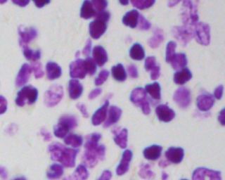

Problem Statement
Classical image processing techniques for nuclei detection work decently well, but they can
perform poorly when nuclei have unusual shapes or are more difficult to distinguish (e.g. in
tissue samples). In some cases, biologists have to manually label the nuclei, which can be both
tedious and laborious. In this project, our goal is to create an algorithm that automatically
identifies nuclei within a cell. What makes this image segmentation task challenging is the wide
variety of nuclei that exist and type of conditions the images can be in. In creating one model,
we will need to ensure it generalises well to different kinds of stains, species, and microscopes.
Moreover, in some instances the nuclei overlap, so during preprocessing we will have to devise
a way to split the nuclei into distinct entities.

It is common in image identification and segmentation problems generally to use convolutional
neural-networks as the architecture of choice, and it is also the approach the academic
community typically uses for problems of biomedical image segmentation specifically. In this
project, I intend to implement various deep learning models and feature engineering techniques
with the purpose of identifying nuclei in images of cells. The two main models I plan on
experimenting with are multilayer perceptron models (MLP) and convolutional neural networks
(CNN).

The theoretical workflow for our problem can be summarised as follows. First, we will undertake
a data exploration to get a better sense of the characteristics of our data and will keep this
information in mind when assessing the performance of our various networks. We will then
construct a simple MLP model and iterate on it by applying different feature engineering
techniques to see how it affects performance of the model. Next, we will repeat a similar
process but using CNNs instead and tweak the parameters to try and improve the performance
of our network, and apply the same feature engineering techniques. We will also implement a
mask prediction technique that does not involve the use of neural networks at all and compare it
to the performance of the deep learning approaches. We will then compare the performance of
all of these different approaches and draw conclusions on what seemed to work best for this
specific problem, and what didn’t seem to have a beneficial effect. We will evaluate the
performance of the network by evaluating the mean average precision at different intersection
over union (IoU) thresholds, which is a way to compare the similarity and diversity of sets
defined as the quotient of the intersection and the union of two sets. As mentioned above, we
will define success as achieving a score of 0.2 for the mean of the average precisions of each
image in the test dataset. We expect that performing some feature engineering before feeding
the images into our network will improve performance, and that more complex CNNs will
outperform much simpler MLP networks.

Metrics
Our aforementioned evaluation metric will be the mean average precision at different
Intersection over Union thresholds, as specified in the evaluation portion of the Kaggle
competition2. This is an appropriate metric to use since our network will be trying to identify
spatial similarity in regions of images. The IoU of a set of pixels in an image and a predicted set
                                                                 A∩B
of pixels to identify an object is calculated as: I oU (A, B ) = A∪B . The metric we will use will then
calculate the precision at a number of different thresholds, starting at 0.5 and increasing by 0.05
to 0.95. The precision value is calculated at each threshold based on the number of false
positives, true positives, and false negatives obtained from comparing the predictions to reality,
                                          T P (t)
using the equation for precision: T P (t)+F P (t)+F N (t) . When a predicted object matches reality with
an IoU above the given threshold, a true positive will be tallied; when a predicted object doesn’t
match reality, a false positive will be tallied; when a real object doesn’t match a predicted object,
a false negative will be tallied. Using these tallies, we will then calculate the average precision of
a single image as the average of the precision values at each IoU threshold, given by:
      1               T P (t)
|thresholds|   ∑ T P (t)+F P (t)+F N (t) . The final metric will be the mean of the average precisions of each
               t
image in the test dataset.

II. Analysis

Data Exploration
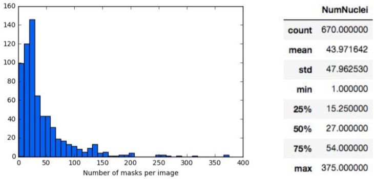
The dataset for this project consists of 670 images with 29,451 individual masks in the training
set, and 65 images in the testing set. To better understand our problem space, we should first
calculate some summary statistics of our data. The first question we should ask is how many
masks are there per image:

2
    See ​https://www.kaggle.com/c/data-science-bowl-2018#evaluation

The distribution of masks per image is skewed to the right with a mean of 44 masks (individual
nuclei) per image and standard deviation of 48. There are some images with as many masks as
375, which may prove difficult for the network to accurately identify the individual nuclei.

Another important question is what the dimensions of the images are. This information can be
found in the image below:

Roughly 550 of the images have similar dimensions. The distribution of image area pixels is
skewed to the right with a mean of 154,758px​2​ and standard deviation of 190,825px​2​. The image
with the greatest proportions has a pixel area of 1,443,520px​2​. Having a wide variety in the pixel
area of the images could have adverse effects on the performance of certain neural network
architectures. However, since we’re creating an algorithm that generalises well, it will need to
perform well on images with varying pixel-area. In the next section, a sample of the dataset has
been provided.

Exploratory Visualization
The more exposure that the network has to a modality of the nuclei image, the more adept it will
be at identifying nuclei in one type of image from another. For this reason, we thought it would
be important to look at the frequency of the different modalities of the images in our dataset. In
his Kaggle kernel, the creator of the competition Allen Goodman3 helpfully already separated
the images by computing the sum of their intensities to create five classes based on the hue of
the background and foreground of the image. He found the following categorical distribution of
images: white foreground and black background (599), black foreground and white background
(16), purple background and purple foreground (71), purple foreground and white background
(41), purple foreground and yellow background (8). We would anticipate that our model would
be better at recognising nuclei in images with a white foreground and black background and
worse at those with a purple foreground and yellow background. Examples of images with these
different modalities can be found below:

3
    Full discussion can be found here: ​https://www.kaggle.com/c/data-science-bowl-2018/discussion/48130

Algorithms and Techniques
As mentioned above, the two main models we will be experimenting with are multilayer
perceptron models (MLP) and convolutional neural networks (CNN). A multilayer perceptron is a
basic type of fully connected neural network, consisting of an input layer, at least 1 hidden layer,
and an output layer. All nodes aside from the input nodes take an activation function which
determines the output of that node. The advantage of using an MLP is that it’s simple, intuitive,
and relatively quick to train - the drawback is that it’s highly prone to overfitting and doesn’t
perform as well as other more complex neural network architectures.

Convolutional neural networks assume that the inputs being received are images.4 What makes
them different from other neural networks is the presence of the convolutional layer, which
contains a filter that slides across the image, taking the dot product of the filter and the portions
of the input image. It also often contains a pooling layer which condenses the information
gathered by the convolutional layer in order to minimize the computational power and number of

4
 This explanation of convolutional neural networks is inspired by:
https://cs231n.github.io/convolutional-networks/

parameters required by the network. With this in mind, we believe that a convolutional neural
network approach will be particularly appropriate for the task at hand.

Benchmark
Our benchmark model will be a simple multilayer perceptron neural network to confirm that our
problem is actually solvable. We will evaluate our models against this simple benchmark to
verify that the changes we are making to our network are improving the model performance
relative to a simpler approach. We will additionally use a supporting benchmark that is provided
in the Kaggle competition itself. There is a ‘Stage2 Top left pixel benchmark’ of 0.000,5 however
a benchmark performance of 0.000 would imply that any model that can identify any nuclei
(even if it’s through random noise) would be acceptable. The top performance in the competition
was a score of 0.631, and the lowest was 0.000. For our purposes, we will consider success
achieving a greater score than 0.2 as it would indicate that our network has performed with
some degree of success and it is in line with that of a lot of the other entries in the competition.

III. Methodology

Data Preprocessing
The dataset that’s been provided has already been cleaned and manually checked by a team of
biologists, and there do not appear to be any irregularities in the data. That said, given the
manual process of labeling the nuclei, there is room for human error in the labelling of masks in
the training set. There’s little we can do to remedy any human error in labelling these images
beyond manually labelling roughly all 30,000 nuclei by hand ourselves, but this would be a
tedious process, and indeed would be performed by someone with much less expertise than
those who originally labelled the images. With this in mind, we do not believe there needs to be
any data preprocessing undertaken for this project.

Implementation
The first step we took before creating and testing any neural network architectures was to
create three feature engineering / segmentation techniques. We thought it might be interesting
to see how well the different networks perform when the data had been slightly altered to aid in
segmentation of the nuclei.

The three feature engineering / segmentation techniques we used were: edge detection,
thresholding, and using the Sobel operator. The edge detection method works by identifying the
edges of the nuclei, filling the holes using mathematical morphology, and removing nuclei with
size below a specified threshold. The thresholding technique assumes there is a bimodal

5
    See ​https://www.kaggle.com/c/data-science-bowl-2018/leaderboard

distribution of grayscale values that can be used to mask out the background and extract the
connected objects. An example of what this this thresholding process looks like for an example
image can be found below:

Out of curiosity, we wanted to see how well just using the thresholding technique to identify
masks in the nuclei images would perform. We anticipated that it would work well when the
images have a clear separation from the background (e.g. when images have a white
foreground and black background) but worse when there’s a less clear separation (e.g. when
images have a purple background and purple foreground). It achieved a mean IoU score of
0.257 which was surprising and surpassed our goal of achieving a score of 0.2.

The final feature engineering technique I implemented involved using the Sobel operator,
another edge detection technique. The Sobel operator creates an elevation map of the nuclei to
help distinguish the edges of the nuclei from the background. The purpose of all three of these
techniques is to clarify where the nuclei are for the network so that it’s better able to determine
what is a mask and what is the background of the image.

After ensuring all of the code for the feature engineering / segmentation techniques worked, we
began assembling our actual neural networks. The process for analysing the images involved
first accessing and resizing both the training images and masks and test images so that they
had dimensions of 256px by 256px, as standardising the size of the images will be important for
implementation with a CNN. We then converted our images to grayscale to simplify the process
of training the network, as there was a great deal of variability in the modality of the images we
were inspecting. After training the model, the output needed to be run-length-encoded6, which
means that we needed to submit pairs of values that contained a start position and run length
for the masks. As an example, ‘12 6’ would mean starting at pixel 12 and running a total of 6
pixels. The reason for submission file being run-length encoded was to reduce the submission
file size.

6
 This is discussed in the submission portion of the competition:
https://www.kaggle.com/c/data-science-bowl-2018#evaluation

I originally started by implementing an MLP with 5 dense layers, halving the number of nodes in
each layer as it progressed. I found that after 2 epochs, the accuracy score was identical for
each additional epoch, and that the model was encoding straight-line pixel values across the
entire image which intuitively seemed very wrong. After tweaking the model, I settled on
simplifying the MLP by reducing the number of dense layers to 2 and adding a dropout layer
between the input and output layers to prevent the model from overfitting; this will be our
benchmark model. After some experimentation with the activation functions for my dense layers
and the optimizer for the model, I found that the best performing activation functions were ‘relu’
in the input layer, ‘sigmoid’ in the output layer, and the best optimizer was ‘adam’. The simple
MLP achieved a score of 0.011 which is very poor - indeed worse than what we achieved
through thresholding alone.

I was concerned about the time it would take to train these models on my personal computer, so
I went to my University’s computer science department and ran the models on their machines.
The slight drawback is they have slightly outdated versions of keras and matplotlib installed (I
believe versions 1.0 or 1.1), but I did eventually get the code to compile using legacy
documentation available online. In the next section, I’ll detail the refinement process I undertook
to select the best possible model.

Refinement
As mentioned in the previous section, the initial solution we devised was a very simple MLP with
2 layers and a dropout layer, achieving a score of 0.011. To improve upon this, I applied the
three feature engineering / segmentation techniques discussed earlier to the data. To recap, the
three techniques I used to improve the performance of the MLP were edge detection,
thresholding, and using the Sobel operator.

Applying edge detection to the data improved the performance of my MLP very very marginally
from 0.011 to 0.012. The edge detection algorithm I employed may have found a bimodal
separation that the MLP was already picking up on, which is why the performance only
improved marginally. This method is not particularly robust, as if a pixel from the mask is missed
then the mask won’t be properly filled; in spite of this, it is good to see that it lead to an improved
result.

Thresholding improved it much more substantially, boosting the performance of the model to
0.039, though this is still a much lower score than what was achieved with thresholding alone. It
must be the case that for many images in our dataset, it is possible to reasonably separate the
masks from the background.

Confoundingly, applying the Sobel operator to the data resulted in a score of 0.000. I attempted
to rectify any errors in my code and resubmitted to the competition and again achieved a score
of 0.000. I hypothesise that the elevation map created by the Sobel operator reduced the

intensity of the nuclei in the centers and made it difficult for the MLP to identify what was
background and what was a mask.

Although applying the feature engineering / segmentation techniques to the MLP increased
performance in 2 out of the 3 cases, the results for the simple MLP network remain quite poor.
As such, I began experimenting with CNN architectures to see how they might perform in
comparison.

I first ran a very basic CNN inspired by a Kaggle kernel by Kevin Mader7 on my personal
computer with a more up to date version of keras, and it achieved a score of 0.152. When I
attempted to run this model on my University’s computer science department machines, I had to
remove the dilation rate parameter from the model as it was only supported in later versions of
keras. I then altered the architecture of the network by adding more layers, and it achieved a
score of 0.072. I originally wasn’t certain if this decrease in performance was due to the
omission of the dilation rate parameter or if it was due to the increase in hidden layers. I then
tried running the same CNN with 30 epochs instead of 10 and found that it improved
performance to 0.094. To confirm whether increasing the number of nodes made the network
perform less well, I kept the number of epochs the same and decreased the number of nodes,
achieving a score of 0.053. The intuition that I gained from this process was that increasing the
training time (by increasing the number of epochs) and the complexity of the model (by
increasing the number of hidden layers) seemed to improve performance.

IV. Results

Model Evaluation and Validation
Following the refinement process, I looked at the performance of all of the models I had created
and submitted. My best performing submission was made by simply using Otsu thresholding as
discussed in Task 3, achieving a score of 0.257. The simple CNN I ran on my personal
computer with a more up to date version of keras and a dilation parameter achieved a score of
0.152. From there, my scores fell quite dramatically. A simple MLP network achieved only 0.011
without any feature engineering, and at most 0.039 with Otsu thresholding applied to the data.
My subsequent CNN models performed worse than my original CNN, with the model with the
least nodes performing the worst with a score of 0.053 and the model with the most nodes and
most epochs performing the best with a score of 0.094. My overall conclusion is that complex
convolutional neural networks seem to perform much better than simpler multilayer perceptron
models in image recognition tasks.

7
 Kaggle kernel by Kevin Mader ‘nuclei overview to submission’,
https://www.kaggle.com/kmader/nuclei-overview-to-submission

To test the robustness of our best performing model, which was simply using Otsu thresholding,
I decided to augment the data by rotating it both 90 and 180 degrees and seeing how the model
performed. Perhaps unsurprisingly, given that the Otsu thresholding technique would likely be
unaffected by the orientation of the scans since it’s only looking at the distribution of grayscale
values in an image, it did not affect its performance. This implies that this technique is fairly
robust to small changes in the orientation of the scans, which is a good thing. However, there is
very little that can be done to improve the performance of this technique, unlike a neural
network - so while it is the best performing approach I was able to take, this is clearly not
generally true as many other participants were successful in creating much more complex
architectures that were better able to solve the problem.

Justification
The benchmark we used for this project was a very simple MLP model that performed with a
score of 0.011, and our best performing model, using Otsu thresholding, managed to achieve a
score of 0.257. We also originally defined success as achieving a score of 0.2 or higher. With
these things in mind, we could say that we have constructed a model that exceeded the
performance of our benchmark and is a workable solution.

That said, the performance of 0.257 is still quite low compared to a lot of participants in the
competition, and there’s no obvious way to improve upon the performance of this technique
since it is not a complex neural network architecture with adjustable parameters. If we are
considering only the predefined way that we chose to define success, and to compare our
solution to the benchmark, then it is fair to say that we solved the problem. However, it would be
unfair to say that it is the best possible solution to the problem that exists. As we will discuss
later in the improvement portion of the project, there is much scope to explore other more
complicated forms of neural networks for problems of biomedical image segmentation.

V. Conclusion

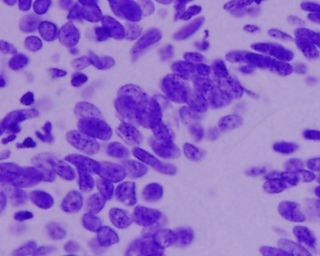
Free-Form Visualization

       Image with sparse nuclei                               Image with dense nuclei

One important aspect of this project that shouldn’t be overlooked is how the density of the nuclei
in an image can affect the performance of the network or image segmentation approach. This is
especially true for the Otsu-thresholding technique that we implemented, where it uses a
bimodal distribution of grayscale values to separate the background from the object of interest.

In the first image where the nuclei are fairly sparse, there is a fairly clear distinction between
what is the background part of the image and what is the nuclei part of the image. In this
instance, it would be relatively simple to identify the nuclei from background. In the second
image where the nuclei are more dense, the distinction between background and nuclei may
become more convoluted, not only due to the ratio of nuclei to background being much higher,
but also due to greater variation in the darkness of the nuclei themselves. In this case, it would
be much more challenging to separate the two.

Reflection
This project involved first exploring the features of the cell scans (e.g. their modality, number of
nuclei per image), implementing feature engineering / segmentation techniques, and finally
constructing deep learning models to automatically identify what parts of each scan was
background and what were nuclei.

One particularly interesting part of the project was understanding the diversity in the
characteristics of cell scans that biologists have to manually identify, and developing a greater
appreciation for the amount of work that biologists put in to manually annotating these scans.
The automation of nuclei identification using machine learning techniques could save biologists
a huge chunk of time, allowing them to focus their efforts more on researching cures for
diseases or other more productive tasks.

One surprisingly difficult part of this project was debugging and getting the code to compile
when using different versions of the python data science packages (i.e. old vs new versions of
tensorflow). Albeit frustrating, it was good to get more practical experience dealing with this type
of problems that is more likely to arise when working in industry. The final model we constructed
does do a decent job of identifying nuclei, and wouldn’t be a bad supplement for a biologist
trying to annotate scans of nuclei, but it should not be fully relied upon and perhaps only
employed when the scans in question have a distinct difference between the background and
foreground colours.

Improvement
The next steps I would take to improve upon this project would be to implement both the
common U-net CNN architecture as is available in the Kaggle competition kernels to measure
its performance against a more simple CNN. I would additionally implement the RCNN model
created by the Kaggler in 1st place in the competition, Allen Goodman, to compare its
performance to the archetypal U-net architecture used for biomedical image segmentation. Both
of these models are substantially more complex than the simple CNN approach I employed in
this project; the main reason I chose not to experiment them in this project was that I did not feel
completely comfortable in my ability to understand how they work and how to properly
implement them. It’s clear that these models would improve performance, and from the Kaggle
leaderboard it is apparent that a better solution than the one I found exists. Nevertheless, the
model I created did surpass the benchmark and appeared to do a decent job at identifying
nuclei in these scans of cells.

References
G. Folego, O. Gomes and A. Rocha, "From impressionism to expressionism: Automatically
identifying van Gogh's paintings," ​2016 IEEE International Conference on Image Processing
(ICIP)​, Phoenix, AZ, 2016, pp. 141-145.

Gatys, L.A., Ecker, A.S., Bethge, M.. “A neural algorithm of artistic style”. arXiv preprint
arXiv:1508.06576 (2015).

Jacobsen, Robert C. and Nielsen, Morten. “Robustness of digital artist authentication.”
Department of Mathematical Sciences: Aalborg University (2011).

Johnson Jr, C. Richard, et al. "Image processing for artist identification." Signal Processing
Magazine, IEEE 25.4 (2008): 37-48.

Khan, Fahad Shahbaz, et al. "Painting-91: a large scale database for computational painting
categorization." Machine vision and applications 25.6 (2014): 1385-1397.

Mordvintsev, A, Olah, C, Tyka, M. “Inceptionism: Going Deeper into Neural Networks“ ​Google
Research Blog​. Available at:
https://research.googleblog.com/2015/06/inceptionism-going-deeper-into-neural.html​ [Accesed
4 Jan. 2018]