Shedding Light on the Weather
←
→
Page content transcription
If your browser does not render page correctly, please read the page content below
Shedding Light on the Weather∗
Srinivasa G. Narasimhan and Shree K. Nayar
Computer Science Dept., Columbia University, New York, USA
E-mail: {srinivas, nayar}@cs.columbia.edu
Abstract
Virtually all methods in image processing and computer
vision, for removing weather effects from images, as-
sume single scattering of light by particles in the atmo-
sphere. In reality, multiple scattering effects are signif-
icant. A common manifestation of multiple scattering
is the appearance of glows around light sources in bad
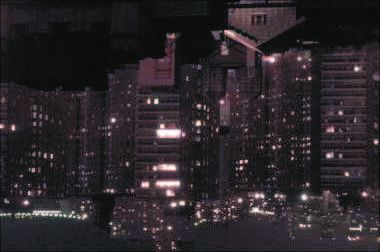
weather. Modeling multiple scattering is critical to un- Figure 1: Night image of light sources in mist. The glows
derstanding the complex effects of weather on images, around sources can reveal the weather condition as well as
and hence essential for improving the performance of the relative depths and shapes of sources.
outdoor vision systems.
Atmosphere Glow in Image
We develop a new physics-based model for the multiple Multiple Scattered Plane
scattering of light rays as they travel from a source to an Light
observer. This model is valid for various weather con-
ditions including fog, haze, mist and rain. Our model
Pinhole
enables us to recover from a single image the shapes and Light Source Unscattered Light
depths of sources in the scene. In addition, the weather
condition and the visibility of the atmosphere can be
estimated. These quantities can, in turn, be used to re- Figure 2: Multiple scattering of light from a source to a
move the glows of sources to obtain a clear picture of sensor results in an image with a glow around the source.
the scene. Based on these results, we demonstrate that a The complexity of modeling the traversal of light rays
camera observing a distant source can serve as a “visual through the atmosphere is well known. One approach
weather meter”. The model and techniques described in to solve this problem is to assume the paths of light
this paper can also be used to analyze scattering in other traversal to be random and then to apply numerical
media, such as fluids and tissues. Therefore, in addi- Monte-Carlo techniques for ray tracing [2]. Computer
tion to vision in bad weather, our work has implications graphics researchers [11; 16] have followed this approach
for medical and underwater imaging. (as well as approximations [7] like diffusion and single
scattering) to render scenes in scattering media. How-
1 Scattering from Light Sources ever, millions of rays must be traced through the atmo-
Recently, there has been growing interest in the vi- sphere to accurately model multiple scattering. Clearly,
sion and image processing communities regarding im- the computational complexity of this approach is too
age understanding in bad weather. Algorithms have high to be suitable for most vision applications.
been developed to recover 3D scene structure [14] and A different approach for modeling light scattering is the
to restore clear day scene contrasts [15] and colors [14; physics-based theory of radiative transfer [3; 6]. The
17] from bad weather images. Most of this work, how- key idea in this approach is to investigate the difference
ever, assumes that the irradiance at any pixel is solely between light incident on, and exiting from, an infinites-
due to scattering within a small column of the atmo- imal volume of the medium, as shown in figure 3. Math-
sphere along the pixel’s line of sight. Figure 1 shows ematically, the change in flux through a small volume
glows around light sources on a misty night. Light is given by an integro-differential equation, called the
from the sources gets scattered multiple times and Radiative Transfer Equation (RTE). The directional in-
reaches the observer from different directions (figure 2). tensity at any location in the atmosphere is then ob-
Clearly, multiple scattering of light must be modeled to tained by solving this equation. The exact nature of the
better understand and exploit weather effects for im- RTE depends on the locations of the radiation sources
proving the performance of outdoor vision systems. and the types and distributions of particles within the
∗ This work was supported by a DARPA HumanID Contract
medium. Nevertheless, RTEs present a clean framework
(N000-14-00-1-0916) and an NSF Award (IIS-99-87979). for describing multiple light scattering.
Proceedings of the 2003 IEEE Computer Society Conference on Computer Vision and Pattern Recognition (CVPR’03)
1063-6919/03 $17.00 © 2003 IEEE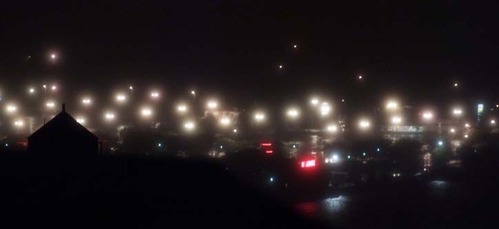
Infinitesimal Element                                                   P( cos α )      (θ,φ )
                                  of the Atmosphere
                                                                                     Incident Light           α
                                                        Exiting Light                   ( θ’ , φ’ )
                                                          Radiance
                                                                                                       Scatterer
                                                                            Figure 4: The phase function P (cos α) is the angular scat-
                    Light Incident
                                                                            tering distribution of a particle. For most atmospheric con-
                 from all Directions                                        ditions, P is symmetric about the incident light direction.
                                                                            The exact shape of P depends on the size of the scatterer,
         Figure 3: An infinitesimal volume of the atmosphere illu-           and hence the weather condition.
         minated from all directions. The radiative transfer equation
         (RTE) [3] describes the relationship between scattered light                      Small
                                                                                  Air                  Haze Mist Fog Rain
         radiance (in a particular direction) and the irradiance inci-                    Aerosols
         dent (from all directions) for the infinitesimal volume.                                                                      q
                                                                               0.0 0.2       0.4      0.7 0.8          0.9     1.0
         In this work, we present an analysis of how light sources
         appear in bad weather and what their appearances re-               Figure 5: The approximate forward scattering parameter q
         veal about the atmosphere and the scene itself. For                of the Henyey-Greenstein phase function for various weather
         this, we first model multiple scattering from an isotropic          conditions. Note that the boundaries between the weather
         point light source using an RTE, and solve it to ob-               conditions are not clearly defined.
         tain an analytical expression for the glow around the              is denoted by P (θ, φ; θ , φ ) and it specifies the normal-
         source. In deriving this expression, we assume that                ized scattered radiance in the direction (θ, φ) for the
         the atmosphere is homogeneous and infinite in extent.               incident irradiance from (θ , φ ). For most atmospheric
         Unlike previous work on RTEs of this type [3; 8; 1;                conditions, the phase function is known to be symmetric
         4], our model is general and is applicable to a variety            about the direction of incident light [3]. So, P depends
         of weather conditions such as haze, fog, mist and rain.            only on the angle α between the directions of incident
         The glow around a point source can be termed as the at-            and scattered radiation (see figure 4), determined as:
         mospheric point spread function of the source. We show
         that the shape of this point spread function depends on                cos α = µµ + (1 − µ2 )(1 − µ 2 ) cos(φ − φ ) , (1)
         the atmospheric condition, the source intensity, and the
         depth of the source from the observer. Then, we de-                where, µ = cos θ and µ = cos θ .
         scribe the glows around light sources of arbitrary sizes,          The exact shape of the phase function depends on the
         shapes, and intensities. It turns out that our model               size of the scattering particle, and hence the type of
         for the glow can be used to efficiently render realistic             weather condition [5]. For instance, phase functions of
         appearances of light sources in bad weather.                       small particles (say, air molecules) have a small peak in
         From a computer vision perspective, it is more inter-              the direction of incidence. Isotropic [P (cos α) = con-
         esting to explore how our model can be used to recover             stant] and Rayleigh [P (cos α) = 3/4(1 + cos2 α)] phase
         information about the scene and the atmosphere. From               functions describe the scattering from air molecules. On
         a single image taken at night, we compute (a) the type             the other hand, phase functions of large particles (say,
         of weather condition, (b) the “visibility” or meteoro-             fog) have a strong peak in the direction of light in-
         logical range, and (c) the relative depths of sources and          cidence. A more general phase function that holds for
         their shapes. In addition, the glows can be removed                particles of various sizes is the Henyey-Greenstein phase
         to create a clear night view of the scene. Although we             function [6]:
         have concentrated on scattering within the atmosphere,                                                    1 − q2
         our model is applicable to other scattering media such                         P (cos α) =                               ,       (2)
                                                                                                       (1 +   q2   − 2q cos α)3/2
         as fluids and tissues.
                                                                            where, q ∈ [0, 1] is the called the forward scattering pa-
         2    Scattering Properties of Weather                              rameter. If q = 0, then the scattering is isotropic, and
         In this section, we discuss the scattering properties of           if q = 1, then all the light is scattered by the particles
         various weather conditions. When light is incident on              in the forward (incident or α = 0) direction. Values for
         a particle, it gets scattered in different directions. This         q between 0 and 1 can generate phase functions of most
         directional distribution of light is called the scattering         weather conditions, as shown in figure 5 [10]. We will
         or phase function of the particle. The phase function              use the Henyey-Greenstein phase function in (2) to an-
                                                                            alyze the glows observed in various weather conditions.

Proceedings of the 2003 IEEE Computer Society Conference on Computer Vision and Pattern Recognition (CVPR’03)
1063-6919/03 $17.00 © 2003 IEEE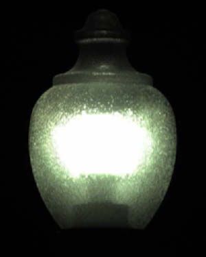
3     The Glow of a Point Source

                                                                                                                       Im
                                                                                                            Pinhole

                                                                                                                        ag
                                                                                                                            eP
         In this section, we derive an analytical expression for

                                                                                                                             la
                                                                                                                        θ

                                                                                                                              ne
         the three-dimensional glow around an isotropic point
         source, that is valid for various weather conditions in-                                                           Measured
         cluding fog, haze, mist, and rain. We call the glow of a                                                            Glow
                                                                                                              Radial
         point source as the Atmospheric Point Spread Function                                                               I (T, µ)
                                                                                                  I0         Depth R
         (APSF). The projection of the APSF onto the image
         plane yields the two-dimensional glow captured by a                                        Isotropic
         camera. Later, we describe the glows around sources of                                    Point Source
         arbitrary shapes and sizes.
                                                                                                 Homogeneous
         3.1     Atmospheric Point Spread Function                                                Atmosphere
         Consider an outdoor environment with a single point                Figure 6: A homogeneous medium with spherical symmetry
         light source immersed in the atmosphere, as shown in               illuminated by an isotropic point source at the center. The
         figure 6. We assume that the source is isotropic i.e.,              scattered radiance is a function of only the radial optical
         the radiant intensity I0 is constant in all directions. A          thickness, T = σR, and the inclination, θ = cos−1 µ , with
         pinhole camera is placed at a distance R from the point            respect to the outward radius vector.
         source. The multiple scattered intensities measured by             with g0 = 0 . The derivation of the above is given in the
         the camera in different directions is the atmospheric               appendix. Lm is the Legendre polynomial of order m,
         point spread function (APSF) of the source.                        and the mth coefficient of the series gm is given by:
         The multiple scattered intensity at a radial distance R
         and at an angle θ with respect to the radial direction,                        gm (T ) = I0 e−βm T −αm log T
         is given by the radiative transport equation (RTE) [3]:                           αm = m + 1
                                                                                                  2m + 1
                     ∂I     1 − µ2 ∂I                                                      βm =             1 − q m−1 .                 (6)
                   µ     +              = −I(T, µ) + . . .                                           m
                     ∂T        T ∂µ
                                                                            In deriving this model, we have assumed that the at-
                        2π +1
                      1                                                     mosphere is homogeneous and infinite in extent. The
                 ...            P (cos α) I(T, µ )dµ dφ .        (3)     function gm (T ) captures the attenuation of light in bad
                     4π
                        0 −1                                                weather, whereas the Legendre polynomial Lm (µ) ex-
                                                                            plains the angular spread of the brightness observed due
         Here, P (cos α) is the phase function of the particles in          to multiple scattering. The glow of a particular weather
         the atmosphere, µ = cos θ and cos α is given by (1).               condition is determined by substituting the correspond-
         T = σR is called the optical thickness of the atmo-                ing forward scattering parameter q (figure 5) in equa-
         sphere. The scale factor σ, called the extinction coeffi-            tion (6). This model is valid for isotropic (q = 0) as
         cient, denotes the fraction of flux lost due to scattering          well as anisotropic (0 < q ≤ 1) scattering, and thus
         within a unit volume of the atmosphere. The “visibil-              describes glows under several weather conditions.
         ity”, V , is related to σ as [10]:
                                                                            Note that the series solution in (5) does not converge
                                      3.912                                 for T ≤ 1. Fortunately, multiple scattering is very small
                                   σ≈       .                       (4)
                                        V                                   for small optical thicknesses [9] and so the glow is not
                                                                            seen. We now make a few observations regarding the
         The intensity I does not depend on the azimuth angle
                                                                            model and show how the shape of the glow varies with
         φ, and hence is said to exhibit spherical symmetry. A
                                                                            the atmospheric condition.
         closed-form solution to the above RTE, for a general
         phase function P (cos α), has not yet been found and is            Angular Spread of Glow and Weather Condi-
         conjectured to be non-existent. However, it is known               tion: Figure 7(a) shows cross-sections of the APSFs
         that most phase functions can be approximated by a                 (normalized to [0 − 1]) for various weather conditions.
         series of Legendre polynomials [3]. By expanding the               The actual three-dimensional APSFs are obtained by
         Henyey-Greenstein phase function (2) in terms of Leg-              rotating the cross-sections about the angle θ = 0 . Re-
         endre polynomials, we show that a series solution to the           call from section 2 that larger the particles, greater the
         above RTE can be obtained as:                                      forward scattering parameter q, and hence narrower or
                                                                            more pointed the glow. For instance, fog produces nar-
                             ∞
                                                                           rower glows than haze. Thus, the spread of the glow
                 I(T, µ) =       (gm (T ) + gm+1 (T )) Lm (µ) ,     (5)
                                                                            can be used for discriminating weather conditions.
                             m=0

Proceedings of the 2003 IEEE Computer Society Conference on Computer Vision and Pattern Recognition (CVPR’03)
1063-6919/03 $17.00 © 2003 IEEE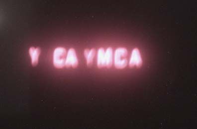
APSF                                         APSF
         1                                           1                                                           Model Coefficients
                                                                              Aerosols, q ~ 0.2                    160
        0.8                                          0.8                        Haze, q ~ 0.75
                                    Haze, q ~ 0.75                                                                 120
        0.6                                          0.6                          Fog, q ~ 0.9
                                                                                                                      80
        0.4 Small Aerosols                           0.4
                                      Fog, q ~ 0.9                                                                    60
              q ~ 0.2
        0.2                                          0.2                                                              30
                                                                                                                      10
        0                                             0                                                                0
              −150 −100 −50   0     50 100 150             −150 −100 −50 0   50 100 150                                    1.02 1.2       1.4   1.6      1.8
               Angle from Radial Direction θ                Angle from Radial Direction θ                                         Optical Thickness T
                              (a)                                     (b)
                                                                                                  Figure 8: Number of coefficients needed in the glow model.
         Figure 7: APSF cross-sections normalized to [0-1] for dif-                               Glows that have a sharp peak (small T ) require a large num-
         ferent weather conditions. (a) Haze produces a wider glow                                ber of terms in the series expansion (5), whereas less than
         than fog but narrower than small aerosols (T = 1.2). (b)                                 10 terms are needed for wide glows (large T ).
         For highly dense atmospheres (T = 4), the glows are wide
         and different weather conditions produce similar APSFs.
                                                                                                      Source                     Region of Minimal
         Angular Spread of Glow and Weather Density:                                                                             Multiple Scattering           Imaging Plane
                                                                                                                  θ
         Figure 7(b) shows the APSFs for highly dense weather
         conditions. As the density of the particles in the atmo-                                                                     R                FOV, δ
         sphere increases, the extinction coefficient σ, and hence
         optical thickness T , increase. For dense atmospheres,                                                                                           Pinhole
         the glows are wide, and the shapes of glows for different                                     Region of Significant
         weather conditions look similar.                                                              Multiple Scattering                                     Image of Glow
         Number of Coefficients (m) in the APSF: Figure
         8 plots the number of coefficients m needed in the series                                  Figure 9: Multiple scattering model for large distances and
         (5) of the APSF, as a function of optical thickness T .                                  small fields of view. The intensities captured by a camera is
         Narrow glows (T close to 1) require a large number of                                    approximated by multiple scattering within a small sphere
         coefficients in the series (5). On the other hand, wide                                    around the source multiplied by constant attenuation from
                                                                                                  the sphere boundary to the pinhole.
         glows require less than 10 coefficients.
         3.2         Small Field of View Approximation
         We derived the APSF keeping in mind a pinhole cam-
         era with a wide field of view. However, if a source and
         its glow are imaged from a large distance with a zoom
         lens (or an orthographic camera with scaling), the field
         of view of the source is very small (usually < 1o ). In-
         tensities from most directions are cut-off by the lens
         optics. Furthermore, the magnitude of multiple scat-                                                    (a)                                       (b)
         tered light is relatively small for large distances. Figure                                              1 APSF
         9 illustrates this scenario. In such cases, we approxi-                                                 0.8
         mate the glow by multiple scattering (see (5)) within
         a small region (sphere) of the atmosphere surrounding                                                   0.6
         the source multiplied by a constant attenuation factor
         (e−T /R2 ). The size of this sphere corresponds to the                                                  0.4
                                                                                                                           Computed                   Measured
         extent of the glow visible in the image. Note that the                                                             APSF                       APSF
                                                                                                                 0.2
         angle θ = cos−1 µ for which we compute multiple scat-
         tering intensity, is once again defined as the inclination                                                0
                                                                                                                           -72    -36     0       36      72
         to the radius vector of the sphere centered at the source.                                                          Angle from Radial Direction θ

         We verified this model using images of distant sources                                                                            (c)
         and their glows with a high dynamic range (12-bits                                       Figure 10: Verification of the glow model. (a) Image of a
                                                                                                  distant point source and its glow. (b) Iso-brightness con-
         per pixel) Kodak digital camera. Weather data from
                                                                                                  tours of the image showing roughly concentric rings. (c)
         a weather web site was obtained at the time of im-                                       Comparison between measured and computed APSFs.

Proceedings of the 2003 IEEE Computer Society Conference on Computer Vision and Pattern Recognition (CVPR’03)
1063-6919/03 $17.00 © 2003 IEEE
age acquisition (rain, q ≈ 0.95 , 2.25 miles visibility).
         The source was about 1 km away from the sensor and
         the field of view was 0.5o . The APSF measured from
         the image of the glow of one of the sources, and the
         APSF computed using our model are shown in figure
         10. The comparison between the measured and com-
         puted APSFs shows the accuracy of our model.

         4     Sources of Arbitrary Sizes and Shapes                                    (a) A street lamp (b) Simulated glow

         Hitherto, we discussed the glow (APSF) of a point
         source seen through the atmosphere. However, sources
         in the real world such as street lamps, can have various
         shapes and sizes. We now extend the APSF to model                        (c) Synthetic sources          (d) Simulated glows
         the glows around sources of arbitrary shapes and sizes.
                                                                              Figure 11: Rendering glows around sources in heavy mist
         Sources of arbitrary shapes and sizes can be assumed                 and rain. The APSF used to render the glows was measured
         to be made up of several isotropic source elements with              from an actual distant source under similar atmospheric con-
         varying radiant intensities I0 (x, y)1 . Then, by the prin-          ditions (see figure 10).
         ciple of superposition of light (we assume the source el-
         ements are incoherent), the intensities due to different
         source elements can be added to yield the total inten-
         sity due to the light source. We assume that the entire
         area of the source is at roughly the same depth from an
         observer. Then, the light originating from each source
         element passes through the same atmosphere. There-
         fore, the image of a light source of arbitrary shape and
         size can be written as a convolution:                                (a) Clear image       (b) Rainy image      (c) Foggy image

                             I = (I0 S) ∗ AP SF .                      (7)

         S is a characteristic shape function that is constant over
         the extent of the light source (not including the glow).
         Since the APSF is rotationally symmetric, the above
         2D convolution can be replaced by two 1D convolu-
         tions making it faster to render sources in bad weather.
         Figure 11 shows two sources and their simulated glows.                    (d) Hazy image     (e) Image through small aerosols
         The APSF used to convolve the source images was ob-                  Figure 12: When can source shapes be detected? (a) Clear
         tained from the real data shown in figure 10(c).                      image of a coil shaped source. APSFs of different weather
                                                                              conditions with the same optical thickness, are applied to
         4.1     Recovering Source Shape and APSF                             this source to obtain their glow appearances. (b) Shape can
                                                                              be roughly detected. (c)-(e) Hard to detect source shape.
         Consider an image of an area source in bad weather.
         From (7), we see that the simultaneous recovery of the               under mild weather conditions. We conclude that it
         APSF and the clear night view of the source (I0 S) is ill-           is easier to detect shapes in rain than in fog, haze or
         defined. However, under certain conditions, the shape                 weather conditions arising due to small aerosols.
         of the source S can be roughly detected despite the
         glow around it. Note that any APSF has a peak at the                 An approach for recovering source shape, and hence
         center that is mainly due to the light scattered in the              for removing the glow around the source, is to use the
         direction of the camera (θ = 0). If this peak has much               APSF computed from real data. Images of two sources
         higher value than the values of neighboring directions,              with different radiant intensities, shown in figure 13(a)
         the actual source location in the image can be roughly               and (d), were captured on the same night. These
         detected using thresholding or high pass filtering. Fig-              sources were adjacent to one another (same depth from
         ure 12 shows simulations of an actual coil shaped lamp               the camera), and hence they share the same APSF,
            1 We assume that occlusions due to source elements are not
                                                                              normalized to [0 − 1]. We applied a simple threshold-
         significant [12] and leave a more formal treatment for future work.
                                                                              ing operator to the image in figure 13(a) to obtain the
                                                                              shape S. We assumed that the radiant intensities I0 of

Proceedings of the 2003 IEEE Computer Society Conference on Computer Vision and Pattern Recognition (CVPR’03)
1063-6919/03 $17.00 © 2003 IEEE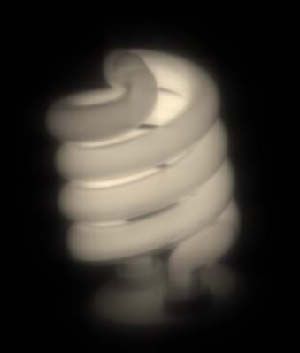
APSF
                                              1                                   6   A Visual Weather Meter
                                             0.8
                                                                                  The ability to compute the type of weather and the
                                             0.6                                  visibility of the atmosphere from one image of a distant
                                                                                  source turns a camera into a “Remote Visual Weather
                                             0.4
                                                                                  Meter”. We performed extensive experiments to test
                                             0.2                                  the accuracy of our techniques. We used images (figure
                                              0
                                                                          Pixel   14(a)) of a real light source acquired under 45 differ-
                                                  −100   −50   0     50   100
                                                                                  ent atmospheric conditions. These light source images
                    (a)              (b)                           (c)            along with ground truth weather data (type and visibil-
                                                                                  ity) and the actual depth of the source from the sensor,
                                                                                  were obtained from the Columbia Weather and Illumi-
                                                                                  nation Database (WILD) [13].
                                                                                  The APSF and its parameters - optical thickness T and
                                                                                  forward scattering parameter q were computed as de-
                     (d)                                       (e)                scribed before, for each of the 45 conditions. Using the
         Figure 13: Shape detection, APSF computation, and glow                   estimated T and the ground truth depth R, the visibil-
         removal. Two adjacent sources (a) and (d) of different                    ity V was computed from (9). The estimated visibili-
         shapes and intensities imaged under rainy and misty con-                 ties follow the trend of the actual visibility curve (figure
         ditions. (b) The shape of the source in (a) is detected using            14(b)). Similarly, we used the estimates of T and the
         simple thresholding. (c) The APSF of the source in (a) is                ground truth visibilities V to compute the depth R from
         computed using (8). (e) The APSF shown in (c) is used to                 (9). The resulting depths obtained in the 45 trials are
         remove the glow around the electronic billboard (d).                     shown in figure 14(c). The plots are normalized so that
         the source elements are constant across the area of the                  the ground truth depth is 1 unit.
         source and then recovered the normalized APSF using:                     The range of estimates for q in the 45 images were be-
                                                                                  tween 0.75 and 1.0. These conformed to the preva-
                           AP SF = I ∗ (I0 S)−1 .                           (8)   lent weather conditions: haze, mist and rain (figure
         The normalized APSF was used to deconvolve the im-                       14(d)). The ground truth weather data from the WILD
         age of the second source (an electronic billboard) and                   database was collected at an observatory three miles
         remove the glow around the second source.                                away from the location of the source. Hence, some of
                                                                                  the errors in the plots can be attributed to the possible
         5    From APSF to Weather                                                incorrect ground truth data.
         In this section, we explore how our model for the APSF
         can be used to recover the depth of the source as well as                7   Conclusion
         information about the atmosphere. The APSF (5) de-                       Light from sources such as street lamps and lit windows
         pends on two quantities: (a) optical thickness T , which                 is scattered multiple times before reaching an observer.
         is scaled depth, and (b) forward scattering parameter q                  The complex multiple scattering effects give an appear-
         of the weather condition. The optical thickness T is re-                 ance of a glow around the light source in bad weather.
         lated to the visibility V in the atmosphere and distance                 We presented an analytical model for the multiple scat-
         R to the source as [10]:                                                 tering of light traversing through the atmosphere and
                                           3.912                                  showed how the shape of the glow is related to the type
                             T = σR ≈            R.                         (9)   and visibility of the atmospheric condition, as well as
                                             V
                                                                                  the depth and shape of the light source. The model
         Furthermore, the value of the forward scattering param-                  we developed can be used for real-time rendering of
         eter q can be used to find the type of weather condition                  sources in different atmospheric conditions. The glow
         (see figure 5). Given an APSF, it is therefore desirable                  model was further exploited to compute scaled depth,
         to estimate the model parameters T and q. The APSF                       visibility, and the type of weather condition, from a sin-
         can either (a) be directly measured from the image (as                   gle image of a source at night. This allowed a camera
         in figure 10) when the source image lies within a pixel,                  to serve as a “visual weather meter”. In addition to vi-
         or (b) be computed from the image as described in sec-                   sion in bad weather, both the model and the techniques
         tion 4.1, when the image of the source is greater than                   presented here have clear implications for medical and
         a pixel. We then use a standard optimization tool to                     underwater imaging.
         estimate the APSF model parameters, T and q, that
         best fit the measured or computed APSF.

Proceedings of the 2003 IEEE Computer Society Conference on Computer Vision and Pattern Recognition (CVPR’03)
1063-6919/03 $17.00 © 2003 IEEE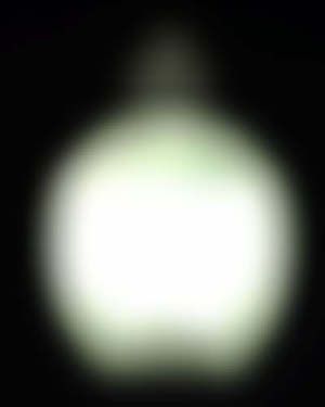
(a) A real light source viewed under 45 different atmospheric conditions.
                                        Miles
                                        5     Ground Truth Visibilities                   Computed Visibilities
                                         4
                                         3
                                         2
                                         1                                                                   Time
                                                    5        10    15    20    25       30     35      40   45

                                                        (b) The accuracy of computed visibilities.
                                        Error
                                          2         Ground Truth Depth               Estimated Depth
                                        1.5
                                         1
                                        0.5
                                         0                                                                   Time
                                                    5       10     15    20    25      30     35       40    45

                                                            (b) The accuracy of computed depth.
                                                                                      Estimated         Groundtruth

                                        Haze
                                        Mist
                                        Rain
                                       Snow                                                                  Time
                                                0       5     10    15    20   25      30     35       40   45
                                                (b) The accuracy of the computed weather condition.
         Figure 14: A Visual Weather Meter: (a) A light source of known shape is observed under a variety of weather conditions
         (rain, mist, haze, snow) and visibilities (1 mile to 5 miles). Optical thickness T and forward scattering parameter q are
         computed from the glow observed in each image. (b) Actual ground truth depth is used to compute the visibility (see (9)).
         (c) To calculate depth, we used the ground truth visibilities and the computed T (see (9)). (d) Weather conditions recovered
         from all images. Empty circle denotes a mismatch between estimated and ground truth weather condition. The images of
         the sources and ground truth data were taken from the Columbia WILD database [13].
         References                                                            [8]   R. E. Marshak. Note on the spherical harmonic method as
         [1]                                                                         applied to the milne problem for a sphere. Physical Review,
               V. Ambartsumian. A point source of light within in a scatter-
                                                                                     71(7), 1947.
               ing medium (translated from Russian by A. Georgiev). Bul-
               letin of the Erevan Astronomical Observatory, 6(3), 1945.       [9]   E. J. McCartney. Optics of the Atmosphere: Scattering by
         [2]   S. Antyufeev. Monte Carlo Method for Solving Inverse Prob-            molecules and particles. John Wiley and Sons, 1975.
               lems of Radiative Transfer. Inverse and Ill-Posed Problems      [10] W. E. K. Middleton. Vision through the Atmosphere. Uni-
               Series, VSP Publishers, 2000.                                        versity of Toronto Press, 1952.
         [3]   S. Chandrasekhar. Radiative Transfer. Dover Publications,       [11] E. Nakamae, K. Kaneda, T. Okamoto, and T. Nishita. A
               Inc., 1960.                                                          lighting model aiming at drive simulators. SIGGRAPH 90.
         [4]   J. P. Elliott. Milne’s problem with a point-source. In Proc.    [12] S. G. Narasimhan and S. K. Nayar. The appearance of a
               Royal Soc. of London. Series A, Mathematical and Physical
                                                                                    light source in bad weather. CU Tech. Report, 2002.
               Sciences, 228(1174), 1955.
         [5]                                                                   [13] S. G. Narasimhan, C. Wang, and S. K. Nayar. All the images
               Van De Hulst. Light Scattering by small Particles. John
               Wiley and Sons, 1957.                                                of an outdoor scene. In Proc. ECCV, 2002.
         [6]   A. Ishimaru. Wave Propagation and Scattering in Random          [14] S.G. Narasimhan and S.K. Nayar. Vision and the atmo-
               Media. IEEE Press, 1997.                                             sphere. IJCV, 48(3):233–254, August 2002.
         [7]   H. W. Jensen, S. R. Marschner, M. Levoy, and P. Hanra-          [15] J. P. Oakley and B. L. Satherley. Improving image quality in
               han. A practical model for subsurface light transport. SIG-          poor visibility conditions using a physical model for degra-
               GRAPH, 2001.                                                         dation. IEEE Trans. on Image Processing, 7, Feb 1998.

Proceedings of the 2003 IEEE Computer Society Conference on Computer Vision and Pattern Recognition (CVPR’03)
1063-6919/03 $17.00 © 2003 IEEE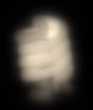
[16] H. Rushmeier and K. Torrence. Zonal method for calculating Let us assume that a solution Im (T, µ) to (16) is a
light intensities in the presence of a participating medium. product of two functions -
SIGGRAPH 87.
[17] Y.Y. Schechner, S.G. Narasimhan, and S.K. Nayar. Instant Im (T, µ) = gm (T )fm (µ) . (17)
dehazing of images using polarization. In Proc. CVPR, 2001.
Substituting into 16, we get,
Solving Spherically Symmetric RTE +1 +1 +1
gm
This appendix provides a sketch of the derivation to gm µQm fm d µ + Lm fm dµ + gm Qm fm dµ
T
solve the RTE (3). More details of the derivation can be −1 −1 −1
found in our technical report [12]. We begin by rewrit- +1 +1
ing the RTE for a spherically symmetric atmosphere, gm
− Qm dµ P (0) (µ, µ ) fm (µ )dµ = 0 . (18)
2 2
∂I 1 − µ ∂I −1 −1
µ + = −I(T, µ) +
∂T T ∂µ
Suppose
2π +1 fm (µ) = Lm−1 + Lm , (19)
1
P (µ, φ; µ φ ) I(T, µ )dµ dφ , (10)
4π for some m > 0. The phase function P can also be
0 −1
expanded using Legendre polynomials:
Integrating P over the azimuth angle, we obtain ∞
2π P (cos Θ) = Wk Lk (cos Θ) . (20)
(0) 1 k=0
P (µ, µ ) = P (cos Θ)dφ . (11) Then, it using (1), it has been shown that [6]
2π
0 ∞
Substituting into equation 10 we get, P (0) (µ, µ ) = Wk Lk (µ)Lk (µ ) . (21)
+1 k=0
∂I 1 − µ2 ∂I 1
µ + = −I(T, µ)+ P (0) (µ, µ ) I(T, µ )dµ , Similarly, we shall expand L k (µ) and µL k (µ) using
∂T T ∂µ 2
−1 Legendre polynomial series:
(12)
L k (µ) = (2k − 1)Lk−1 (µ) + (2k − 5)Lk−3 (µ) + . . .
Let Qm (µ) be a function defined for some m > 0, such
that µL k (µ) = kLk (µ) + (2k − 3)Lk−2 (µ) + . . . . (22)
d((1 − µ2 )Qm (µ)) L m (µ)
Lm (µ) = ⇐⇒ Qm (µ) = . (13) We substitute equations 13, 19, 21 and 22, into equation
dµ m(m + 1) 18 and simplify each term using the orthogonality of
When there is no confusion, we drop the parameters µ Legendre polynomials to get:
and T for brevity. Multiplying 12 by Qm and integrat- g
ing with respect to µ over [−1, +1], we get, g + αm + gβm = 0
T
+1 +1 +1 2m + 1 Wm−1
∂I 1 − µ2 ∂I αm = m + 1 βm = 1− . (23)
µQm dµ + Qm dµ = − Qm I dµ m 2m − 1
∂T T ∂µ
−1 −1 −1 For the Henyey-Greenstein phase function (2), Wk =
+1 +1 (2k + 1) q k [6]. The solution to (23) is,
1
+ Qm dµ P (0) (µ, µ ) I(T, µ )dµ , (14) gm (T ) = I0 e−βm T −αm log T , (24)
2
−1 −1 where the constant of integration I0 is the radiant inten-
sity of the point source. Since we assume that the at-
Using 13, it can be shown that [3],
mosphere is infinite in extent, the above equation auto-
+1 +1 matically satisfies the boundary condition: gm (∞) = 0.
2 ∂I
Qm (1 − µ ) dµ = I(T, µ)Lm dµ . (15) Additional boundary conditions (say, camera is not out-
∂µ door) can be applied if known. For our analysis, we use
−1 −1
the solution to the RTE given by the superposition
Now the RTE can be rewritten as ∞
+1 +1 +1 I(T, µ) = gm (T ) (Lm−1 (µ) + Lm (µ)) . (25)
∂I 1
µQm dµ + Lm I dµ = − Qm Idµ m=1
∂T T
−1 −1 −1 For convenience, we rewrite the above equation as,
+1 +1 ∞
1 (0) I(T, µ) = (gm (T )+gm+1 (T )) Lm (µ) , g0 = 0. (26)
+ Qm (µ)dµ P (µ, µ ) I(T, µ )dµ , (16)
2 m=0
−1 −1
Proceedings of the 2003 IEEE Computer Society Conference on Computer Vision and Pattern Recognition (CVPR’03)
1063-6919/03 $17.00 © 2003 IEEE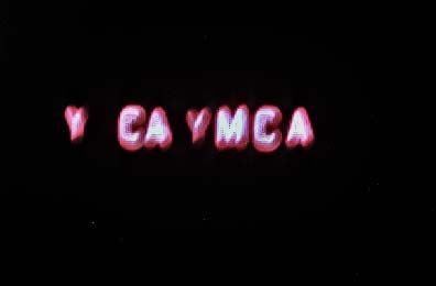
You can also read