A constitutive model for sands: Evaluation of predictive capability Un modelo constitutivo para arenas: Evaluación de capacidad predictiva
←
→
Page content transcription
If your browser does not render page correctly, please read the page content below
A constitutive model for sands: Evaluation of predictive capability
Un modelo constitutivo para arenas: Evaluación de capacidad predictiva
                                                   A. Sfriso
                                            University of Buenos Aires

                                                  RESUMEN
Se presenta un modelo constitutivo que describe el comportamiento mecánico de arenas bajo carga
monotónica dentro del rango de tensiones y deformaciones de interes ingenieril. Utiliza elasticidad
dependiente de la presión, una versión de tres invariantes del criterio de Murata–Miura para compresión
plástica, un criterio de Matsuoka–Nakai extendido para la respuesta inelástica al corte, y una implementación
3D de la teoría tensión – dilatancia de Rowe. Con el fin que el modelo sea útil y atractivo para los ingenieros
geotécnicos, sus ocho parámetros fueros elegidos entre aquellos mejor conocidos por la comunidad
geotécnica. Se presentan algunas simulaciones numéricas que comparan el desempeño del modelo con
resultados experimentales.
Palabras clave: modelos constitutivos, tensión-dilatancia, arenas, ruptura de partículas

                                                 ABSTRACT
A constitutive model to describe the mechanical behavior of sands under monotonic loading throughout the
stress and strain range of engineering interest is presented. The model uses pressure-dependent elasticity, a
three-invariant version of the Murata-Miura yield loci for plastic compression, an enhanced Matsuoka-Nakai
criterion for inelastic shear response, and a 3D implementation of Rowe’s stress-dilatancy theory. In order to
make the model useful and attractive to geotechnical engineers, its eight parameters were selected among
those well known to the geotechnical community. Some numerical simulations are presented to compare the
model’s performance against experimental results.
Keywords: constitutive modeling, strength-dilatancy, sands, particle crushing

1   INTRODUCTION                                           i) different plane strain and triaxial compression fric-
                                                           tion angles; ii) pressure dependent peak friction an-
Computational geomechanics is gaining widespread           gle; iii) effects of particle crushing; iv) different di-
acceptance as a reliable procedure for routine engi-       latancy ratios in compression and extension tests;
neering analysis in both static and cyclic loading         and v) the possibility that a sand specimen has to be
conditions. Mohr-Coulomb and hyperbolic laws are           both heavily overconsolidated and contractive, or
those most used by practitioners to model sand be-         normally consolidated and dilatant.
havior, despite the fact that these models have input          The success of a novel constitutive model de-
parameters that are problem-dependent. For in-             signed for routine analyisis can be ultimately meas-
stance, one set of parameters is used to model the         ured by it’s degree of usage and, by the time it is in-
behavior of the sand surrounding a pile shaft, and a       troduced to the geomechanics community, by its
different set is used to model the pile tip, even if       ease to be understood and accepted. The most im-
shaft and tip rest in the same sand deposit.               portant decision that a model-builder can make to
   Robust and reliable modeling of sand behavior           achieve this objetive is to select few, easily under-
may be better achieved if routine computational ge-        standable input parameters and use well established
omechanics benefits from some improvements in-             formulas wherever applicable.
cluded in advanced models available in the academic            The model presented here is the monotonic subset
environment. These “advanced” features are well-           of a more general constitutive model for sands called
known to practitioners and routinely accounted for         ARENA and developed at the University of Buenos
in hand-made computations. Some of them are:               Aires, Argentina.
2 MODEL FORMULATION 2.2.2 Proportional compression
In a typical oedometer compression test all stresses
grow proportionally, forcing particles to slide, roll
2.1 Elasticity and crush to a more dense packing. The relevant
Isotropic, pressure and void ratio dependent hypo- stress measure is the major principal stress σ1 but, if
elasticity is adopted. Expressions proposed by the stress ratio is known, p can be used as a more
Pestana (Pestana&Whittle 1995) and Hardin (Har- convenient stress measure. In a general compression
din&Richart 1963) were selected because they have test, however, obliquity varies during compression,
material parameters not dependent on pressure or and a cap closure must be used.
void ratio. These are
2.3 Effect of mean pressure on inelastic behavior
m
Both shear and compression behavior depend on
1 + e0 p
K = cb pref mean pressure p, void ratio e and relative density Dr
e0 pref for a given sand. For extreme high stresses, an ulti-
m
(1) mate e - p relationship was determined by Pestana
( ce − e0 ) p
2
(Pestana&Whittle 1995) in the form
G = cs pref
1 + e0 p ref
pult = e−1 ρ pr pref (4)
where K is bulk modulus, G is shear modulus, cb, cs,
ce, and m are material parameters, p is mean pressure where pr and ρ are material parameters. Pestana
and pref is a reference pressure. e0 is the zero-stress (Pestana&Whittle 1995) shows that ρ lies in the
void ratio, obtained by an elastic unload from cur- range 0.36 < ρ < 0.45 for many sands. Because ρ
rent void ratio e to p = 0 KPa. has little influence in the behavior of sands at engi-
neering stress levels, it is accurate enough to take
1− m ρ = 0.40 and define the crushing parameter
1 p
e0 = e exp (2)
cb (1 − m ) pref p e 2.5 p
χ= = 0 (5)
pult pr pref
2.2 Sources of inelasticity Thus, if χ ≪ 1 particle crushing is negligible and
both dilatancy and compression stiffness depend on
The mechanical behavior of sands depends mainly
relative density only. On the other side, if χ ≃ 1 , no
on the resistance of particle contacts to sliding in
dilatancy occurs and compression behavior depends
shear and crushing in compression.
mainly on the strength of the grain material.
While the physical phenomena that governs both
deformation mechanisms are inter-linked and not
2.4 Shear strength
perfectly understood, the conceptual problem can be
splitted for modeling purposes into the effects of
shear at constant mean pressure and proportional 2.4.1 Peak friction angle
compression. Loose sands contract during drained shear until a
critical void ratio ec and a critical friction angle φc
2.2.1 Shear loading are reached (Casagrande 1936, 1975). Dense sands
In a typical triaxial test, deformation in shear is gov- dilate until they reach the same state {ec, φc} but,
erned by the change of stress-ratio, measured in ten- while dilating, the instant mobilized angle of friction
sor r = s p or scalar form r = r . s = σ − pI is the is higher than φc up to a peak value φf.
deviatoric stress tensor, σ is the stress tensor and I is Under high pressure, no dilation occurs and there-
the unit tensor. In general stress space, however, the fore φf = φc (De Beer 1965). Bolton (Bolton 1986)
obliquity of the stress state has no unique definition. took into account the dependency of φf on both stress
One suitable scalar measure is the aperture of the and density through the expression
Matsuoka–Nakai (Matsuoka&Nakai 1974) cone
p
φ f = φc + 3° Dr Q − ln − 3° (6)
r − 3J KPa
2
M = 3 1 2 3r (3)
1 − 2 r + J 3r
Parameter Q accounts for particle strength. Crushing
where J 3r = 13 r ⋅ r : r . For hydrostatic conditions (no resistance of a given sand, however, depends both
shear stress), r = J 3 r = M = 0 . on particle strength and void ratio. This fact can be
better accounted for with the modified expressionφ f = φc − 3° Dr ln [ χ ] − 2° (7) Peak friction angle - Sacramento Sand
Experimental vs. computed results
φ46
Data used by Bolton (Bolton 1986) to calibrate (6) is e02.5 p
44 φ = φc − 3° Dr ln − 2°
matched by (7) within 1.5°. An upper limit for engi- pr pref
neering analysis φmax is obtained by computing (7) 42
φc = 33.5° pr = 40
with the minimun void ratio emin and for a low pres- 40
sure p=100 KPa. Expression (7) predicts φf < φc if 38
36
pr − 2° Dr=38%
p>
34
exp pref (8) Dr=100%
3°Dr
2.5
e0 32
100 1000 p [KPa] 10000
which means that the sample must densify to reach Fig 2. Calibration of (7) for Sacramento sand. Experimental
{ec, φc} . If contraction is impeded, so-called lique- data after Lee, 1967.
faction occurs.
where µ is an internal variable. The plastic strain in-
2.4.2 Failure surface in shear crement in shear εɺ sp = λɺs m s is governed by the non-
φf is a parameter of the Mohr- Coulomb failure associative tensor field (Macari 1989)
criterion. In the present model, the Matsuoka-Nakai
criterion (Matsuoka&Nakai 1974) is adopted and φf n ds
is used to calibrate it. The failure surface in shear is ms = +βI (11)
n ds
µf +6
Ff = r 2 − ( µ f + 9 ) J 3r − µ f = 0 (9) where n ds = n s − 13 n s : II, n s = ∂Fs ∂σ , β is a dila-
2 tancy variable and λs is a plastic multiplier.
where µf = 8 tan2[φf] is a strength parameter that in- 2.5.2 Dilatancy
herits dependence on Dr and χ. β is computed after Rowe’s strength-dilatancy
The selection of a three invariant failure criterion theory (Rowe 1962). Rowe introduced the expres-
like (9) accounts for the difference between plane sion Win Wout = Ncv , Win and Wout being the work
strain and triaxial compression friction angles, done by and against the surrounding media,
whereas it’s calibration using (7) accounts for the Ncv = (1 + sin φ cv ) (1 + sin φ cv ) and φcv the constant-
dependency of peak friction on density and mean volume friction angle.
pressure. Fig. 1 shows the failure surface in shear, Due to deviatoric associativity, ms shares eigen-
while Fig. 2 shows the calibration of (7) for Sacra- vectors with σ, a fact that allows for the computation
mento sand (Lee 1967). of β in their common principal stress space, where
σ →{σ1, σ2, σ3} and ms →{ms1, ms2, ms3}. The ex-
pressions are
W = σ ⋅ m ds = {σ 1msd1 , σ 2 msd2 , σ 3 msd3 }
∑W +N ∑W
WI > 0
cv
WI < 0
(12)
β= I :1… 3
N cv ∑ σ I + ∑ σ I
WI < 0 WI > 0
φcv depends on mineralogy, density and particle
shape. A convenient expression, following concepts
Fig. 1. Curved failure surface in shear, accounting for pressure, by Horne (Horne 1965, 1969) and introduced here is
density and stress – path dependent peak friction angle.
2.5 Shear plasticity φ + (3° Dr ln [ χ ] + 2°) 3
φcv = max c (13)
9 8φc − 8°
2.5.1 Loading surface and dev-plastic strain
The loading surface is the Matsuoka-Nakai cone These expresions account for contractive – dilatant
passing through the current stress state behavior, lower φcv values for dense samples and
low confinement, and a distinct response in triaxial
µ +6 compression, plane strain and triaxial extension.
Fs = r 2 − ( µ + 9 ) J 3r − µ = 0 (10)
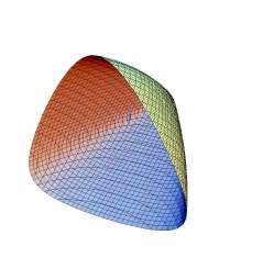
2Fig. 3 shows the dilatancy coefficient β as a func- 2.6 Plastic compression
tion of σ1/σ3 and σ2/σ3 ratios in the range 1 to 5, for
the particular case Ncv = 3.
2.6.1 Yield surface
σ2 σ3 Murata and Miura (Murata&Miura 1989) proposed a
closed yield surface for sands in the low and high
pressure range. It’s expression is
( (σ − σ 3 ) p ) + η1 ln [ p pc ] = 0
2
1 (17)
β
where η1 is a material parameter and pc is the pre-
consolidation pressure. An alternative expression
having a Matsuoka-Nakai shaped cross section, de-
rived from Sfriso (Sfriso 1996), is
σ1 σ 3
Fig. 3. Stress – ratio dependent dilatancy coefficient. Fc = M + η ln [ p pc ] = 0 (18)
2.5.3 Hardening function in shear Fig. 4 shows a trimmed side and a front view of
Duncan-Chang’s hyperbolic law (Duncan&Chang (18). Three slices have been cut from the latter to
1970) for monotonic loading is the most frequently show the complete surface closing towards its apex.
used stress-strain law for sands. Applied to shear
modulus it yields
2
σ1 − σ 3
Gt = Gi 1 − R f (14)
(σ 1 − σ 3 ) f
In (14), Gt is the tangent shear modulus, Gi is the
“static initial” shear modulus, and Rf is the failure ra-
tio (Duncan&Chang 1970, Duncan et al 1980, Nu-
ñez 1995). The hyperbolic law can be adapted to the Fig 4. Partial side view and front view of the cap closure.
Matsuoka-Nakai criterion and converted to a harden-
ing function for primary loading 2.6.2 Plastic strains
Associative cap plasticity is adopted. Plastic strains
2 3 Gt G G in compression are computed using εɺ cp = λɺc m c ,
µɺ = εɺ spd where mc = nc nc , nc = ∂Fc ∂σ and λc is a plastic
µ f 1 + Gt G p s (15) multiplier. While (17) was intended to model both
shear and compression behavior of sands, (18) only
( )
2
Gt = Gi 1 − R f µ µ f serves as a cap closure. To avoid unrealistic dila-
tancy in proportional compression, η is solved out to
In the above expression, Gi is pressure and density yield I : mc = 0 at failure. The expression is
dependent, and a dedicated set of material parame-
µf
ters should be adopted to calibrate it. To avoid these
extra parameters, concepts introduced by Trautmann
η=
12
( 3µ f + µf µ f + 8 + 24 ) (19)
and Kulhawy (Trautmann&Kulhawy 1987) can be
exploited to get the relationships The intersection between the cap closure (18) and
the loading surface (10) is a planar curve entirely
1 + 2Ψ contained in a deviatoric plane in stress space.
Gi = G R f = 0.7 + 0.2Ψ (16)
6
2.6.3 Hardening function in compression
where Ψ = ( tan φ f − tan φ c ) ( tan φ max − tan φ c ) is an in- Relative density dominates low pressure stiffness in
direct measure of stress level and density. Expres- isotropic compression, while particle crushing is the
sions (16) were calibrated to match data by Duncan driving mechanism in the high pressure range (Rob-
(Duncan et al 1980) and Seed (Seed et al 1984). For erts&De Souza 1958, Schultze&Moussa 1961,
instance, a dense sample under low stresses has a Pestana&Whittle 1995). In this model, these two
“initial static” to “elastic” stiffness ratio Gi/G ~ 1/2 stress regions are modeled separately via distinct re-
and a failure ratio Rf ~ 0.9, whereas the same sample duction factors Cl and Ch applied to the elastic bulk
under high stresses shows Gi/G ~ 1/5 and Rf ~ 0.7. stiffness K p = Cl / h K , namelym −1 4 MODEL VALIDATION
2 − Dr c p
Cl = Ch = b −1 (20)
Dr 2.5 pref Fig. 5 shows the predicted vs. measured behavior of
Sacramento river sand in isotropic compression (Lee
where l and h stand for low and high pressure. In- 1967). Adopted parameters are shown in the figure.
termediate response depends on the contribution of
both mechanisms via a weighting function Isotropic compression - Sacramento Sand
Experimental vs. computed results
e
0.90
1 1 emin = 0.61 emax = 1.03
ζ = + erf 2 (1 + Dr )( χ − 1) (21) p = e0−2.5 pr pref
cb = 380 cs = 740
2 2 0.80 ce = 2.17 m = 0.5
pr = 40 φc = 33.5°
Oedometric compression and isotropic compression 0.70 e0 = 0.87,0.78,0.71,0.61
of a given sand yield approximately the same σ1 − εv
curve. This allows for the extension of isotropic 0.60
compression relationships to general stress space.
The adopted hardening function in compression is
0.50
100 1000 10000 p [KPa]
100000
pɺ c = 3
1− ( M M +8 − M ) 6
K εɺ cp (22) Fig. 5. Predicted vs. experimental results for Sacramento river
(1 − ζ ) Cl + ζ Ch sand in isotropic compression. Data from Lee, 1967.
Fig. 6 shows the numerical simultation of oedometer
2.7 Behavior in tension tests of normally consolidated Sacramento river
sand, while Fig. 7 reproduces the simulation of the
No tensile stresses are allowed for. If a strain path
same tests on samples preconsolidated to σ1c = 100
leads to tensile stresses, the response is zero stress,
KPa. While no slope change is observed at σ1c for
zero stiffness and all internal variables are reset.
the densest OC sample, a clear change in overall
2.8 Input parameters stiffness is predicted for the loosest one.
Input parameters are eight: emin and emax, min / max
void ratios needed to compute Dr; cb and m for bulk Oedometric compression - NC behavior
stiffness; cs, ce and m for shear stiffness, φc for criti- 1 10 100 1000 σ1 [KPa]
10000
0.0%
cal state friction angle and pr for particle crushing. σ1c = 0 KPa
Of these, only cb and pr, adopted from Pestana’s
compression model, need some comment. pr can be 0.2%
best calibrated using a series of triaxial compression
tests of dense samples, performed over the maxi-
mum available pressure range, or estimated from 0.4%
Dr=33.3%
available data on the dependence of peak friction Dr=66.6%
angles on mean pressure (see, for instance, Duncan ε1
Dr=100%
0.6%
et al 1980). cb can be readily computed from the re-
bound curve of an oedometer test of a dense sample, Fig. 6. Plaxis simulation of an oedometer test of a normally
where plastic deformations developed during consolidated sample of Sacramento river sand.
unloading are negligible. It can also been estimated
from available data and correlations (see, for in- Oedometric compression - OC behavior
stance, Seed et al 1984). σ1 [KPa]
1 10 100 1000 10000
0.0%
σ1c =100 KPa
3 MODEL IMPLEMMENTATION
0.2%
The model was integrated through a fully implicit,
generalized plasticity algorithm in strain space. De-
tails of the numerical issues have been presented 0.4%
Dr=33.3%
elsewhere (Sfriso 2006a, b). The model was im- Dr=66.6%
plemmented in Plaxis V8.2 as an user-defined ε1
Dr=100%
0.6%
model. The DLL library and user maual is available
for download at www.fi.uba.ar/materias/6408. Fig. 7. Plaxis simulation of an oedometer test of a over con-
solidated sample of Sacramento river sand.Fig. 8 shows the calibration of the model for the REFERENCES
monotonic undrained shearing of Nevada Sand. Data
was obtained from Arulmoni et al (Arulmoni et al Arulmoni, K. et al (1992). VELACS Laboratory testing pro-
1992). Further information can be found elsewhere gram. Soil data report. ETP 90-0562, 77 p.
Bolton, M. (1986). The strength and dilatancy of sands. Geo-
(Sfriso 2006a, b). The difference bewween the pre- technique 36, 1, 65-78.
dicted and observed pore pressure response largely Casagrande, A. (1936). Characteristics of cohesionless soils af-
obeys to water cavitation in the experimental test. fecting the stability of slopes and earth fills. J. Boston Soc.
Civil Engineers, 23 1, 13-32.
3200
Casagrande, A. (1975). Liquefaction and cyclic deformation of
sands - a critical review. V PCSMFE, 1-25. Buenos Aires.
q - Deviatoric stress
2800
2400 De Beer, E. (1965). Influence of the mean normal stress on the
2000 shearing resist. of sand. VI ICSMFE, Montreal, 1, 165-169.
(kPa)
1600 Duncan, J. and C. Chang (1970). Nonlinear analysis of stress
Exp p=80 KPa
1200 Exp p=160 KPa and strain in soils. Journal of Soil Mechanics Foundation
800 Model p=80 KPa
400 Model p=160 KPa
Division, ASCE, 96, SM5, 1629-1653
0 Duncan, J., P. Byrne, K. Wong and P. Mabry (1980). Strength,
0 5 10 15 20 Axial25strain (%)
30 stress-strain and bulk modulus parameters for finite element
analyses of stresses and movements in soil masses. Report
0 5 10 15 20 Axial25strain (%)
30 UCB/GT/80-01, Berkeley, 72 p
Hardin, B. and F. Richart (1963). Elastic wave velocities in
0 granular soils. Journal of Soil Mechanics Foundation Divi-
(u - uo) - PWP
Change (kPa)
-400 sion, ASCE, 89, SM1, 33-65.
-800 Horne, M. (1965). The behaviour of an assembly of rotund,
-1200 rigid, cohessionless particles I, II. Proc. Roy. Soc. London
-1600 A, 286, 68-97.
-2000 Horne, M. (1969). The behaviour of an assembly of rotund,
-2400 rigid, cohessionless particles III. Proc. Roy. Soc. London A,
310, 21-34.
Fig. 8. Predicted and observed behavior of Nevada sand during Lee, K. and H. B. Seed (1967). Drained strength characteris-
undrained shearing. Data from Arulmoni et al, 1992. tics of sands. JSMFD, ASCE, 93, SM6, 117-141.
Macari, E. (1989). Behavior of granular materials in a reduced
gravity environment and under low effective stresses. Ph. D
5 CONCLUSIONS Thesis, U. of Colorado, 177 p.
Matsuoka, H. and T. Nakai (1974). Stress-deformation and
strength characteristics of soil under three different princi-
A constitutive model for the monotonic behavior of pal stresses. Proceedings of Japan Society of Civil Engi-
sands has been presented. The model uses eight ma- neers, 233, 59-70.
terial parameters to account for many aspects that Murata, H., N. Miura, M. Hyodo and N. Yasufuku (1989). Ex-
are not included in other models oriented to routine perimental study on yielding of sands. In: Mechanics of
granular materials, Report ISSMFE TC13, 173-178.
analyses, namely the effect of particle crushing on
Núñez, E. (1995). Propiedades mecánicas de materiales granu-
peak strength and compression stiffness and a 3D lares incoherentes Acad. Nac. de Cs. Ex. Fís. Nat. Bs. As.,
implemmentation of strength – dilatancy theory. 46, .71-89.
The model has been calibrated using widely ac- Pestana, J. and A. Whittle (1995). Compression model for co-
cepted expressions by Hardin (Hardin&Richart hesionless soils. Geotechnique, 45(4), 611-631.
1963), Duncan (Duncan et al 1980) and Seed (Seed Roberts, J. and J. De Souza (1958). The compressibility of
sands, Proceedings ASTM, 58, 1269-1277.
et al 1984). Parameters have been chosen, whenever Rowe, P. (1962). The stress dilatancy relation for static equilib-
possible, among those most accepted by geotechni- rium of an assembly of particles in contact. Proc. Royal
cal engineers. Most of them have large available da- Soc. London, 269, 500-527.
tabases gathered during decades of routine usage. Schultze, E. and A. Moussa (1961). Factors affecting the com-
Despite the relatively few material parameters pressibility of sand, Proceedings V International Confer-
ence on Soil Mechanics and Foundation Engineering, Paris,
used, the model retains an acceptable degree of pre-
I, 335-340.
dictive capability for many problems, including the Seed, H., R. Wong, I. Idriss and K. Tokimatu (1984). Moduli
behavior of foundations and slopes. and damping factors for dynamic analyses of cohesionless
soils. Report UCB/EERC-84/14, Berkeley, 37 p.
Sfriso, A. (1996). Una ecuación constitutiva para arenas. En-
ACKNOWLEDGMENTS cuentro de geotécnicos argentinos GT'96,I, 38-46.
Sfriso, A. (2006a). Calibration of ARENA for Nevada sand
based on VELACS project results. In: VII WCCM, elec-
The writer acknowledges the deep influence that tronic publication, Los Angeles.
Eduardo Núñez, master and advisor, had in this re- Sfriso, A. (2006b). ARENA – Una ecuación constitutiva para
search project through many years of continuous arenas. Dr. Eng. Thesis, sumitted to Univ. of Buenos Aires.
teaching and guidance. Comments and support by E. Trautmann, C. and F. Kulhawy (1987). CUFAD - A Computer
Dvorkin, E. Macari, G. Etse and G. Weber are grate- program for compression and uplift foundation analysis and
design. Report EL-4540-CCM, Vol 16. EPRI, 148 p.
fully recognized.You can also read