Fuel Efficiency of Vehicles from 2004 - Jackie Gushue Yi Wu
←
→
Page content transcription
If your browser does not render page correctly, please read the page content below
Fuel Efficiency of Vehicles from 2004

                               Jackie Gushue
                                       Yi Wu
Introduction There are economic, political, and environmental benefits of more fuel efficient vehicles. With rising gas prices over recent years, the fuel efficiency of vehicles has come under closer scrutiny. It is estimated that consumers could save as much as $1,400 in fuel costs each year by choosing the most fuel efficient vehicle in a particular class. In political terms, more than half of the oil used to produce gasoline is imported. Raising fuel efficiency of vehicles is seen as a viable option in reducing dependency on foreign oil. Greater fuel efficiency can also reduce a person’s carbon footprint. Every gallon of gasoline burned contributes about 20 pounds of carbon dioxide. The difference in carbon emissions between a vehicle that gets 25 miles per gallon and one that gets 20 miles per gallon is about 10 tons of carbon dioxide over a vehicle’s lifetime (fueleconomy.gov). Given the above benefits, we would like to ascertain what variables—structural and non- structural—influence or determine a car model's fuel efficiency. We used a combination of SQL, Python, and data mining techniques to assess these relationships. We found that non-structural do not have a statistically significant influence on fuel efficiency of vehicles whereas structural variables do. Despite this, complex prediction algorithms such as neural networks can make a decent fuel efficiency prediction with using non-structural variables as inputs. Data Our dataset, “2004 New Car and Truck Data,” consists of 428 observations or vehicles and 20 variables that specify the price, fuel efficiency, and structural characteristics (e.g. engine size) of the vehicle. The original dataset comes from the Journal of Statistics Education Data Archive (JSE). The link on JSE’s website is broken; however, the data can be found here: http://www.idvbook.com/teaching-aid/data-sets/2004-cars-and-trucks-data/. A table that summarizes all the variables in the dataset is listed in Table 1. Three additional variables were also added to this dataset (Table 2). We added a model year variable which tells us the year the specific car model was first made. This variable was entered manually and found using Wikipedia. The second variable added is the time period or simply how many years elapsed since the car was first introduced until 2004. This was done using Excel. The third variable added is the country of origin. This variable tells us the country in which a vehicle’s car manufacturer is headquartered. For example, the vehicle “Mercedes-Benz C230 Sport 2dr” would have a country of origin value equal to “Germany.” This variable was added to the dataset using Python. The steps taken will be described in more detail in the next section.
Table 1: 2004 New Car and Truck Data Variables

Variable                          Description
Vehicle                           Name of the vehicle
Small/Sporty/Compact/Large
                                  Binary variable: 1 = yes, 0 = no
Sedan
Sports Car                        Binary variable: 1 = yes, 0 = no
Sport Utility Vehicle (SUV)       Binary variable: 1 = yes, 0 = no
Station Wagon                     Binary variable: 1 = yes, 0 = no
Minivan                           Binary variable: 1 = yes, 0 = no
Truck                             Binary variable: 1 = yes, 0 = no
All-Wheel Drive                   Binary variable: 1 = yes, 0 = no
Rear-Wheel Drive                  Binary variable: 1 = yes, 0 = no
                                  What the manufacturer thinks the vehicle is worth,
Suggested Retail Price            including adequate profit for the
                                  automaker and the dealer (U.S. Dollars)
                                  What the dealership pays the manufacturer (U.S.
Dealer Cost
                                  Dollars)
Engine Size                       Size of engine (liters)
Cylinders                         Number of cylinders (1 if rotary engine)
Horsepower                        Horsepower of vehicle
                                  Number of miles per gallon a vehicle gets if driving in
City Miles per Gallon
                                  the city or in stop-and-go traffic
                                  Number of miles per gallon a vehicle gets if driving on
Highway Miles per Gallon
                                  highways or roads with continuous traffic flow
Weight                            Weight of vehicle (pounds)
Wheel Base                        Size of wheel (inches)
Length                            Length of vehicle (inches)
Width                             Width of vehicle (inches)
Table 2: Added Variables Variable Description Model Year Year car model was first made Time Period Number of years elapsed since car model was first introduced Country of Origin Country in which a vehicle’s car manufacturer is headquartered Data Preparation Data Table Formation After the model year variable was manually entered into the original data file and the time period calculated, python code was written to automate the process of assigning the country of origin values. The finalized python code reads in the data file and writes a new data file that includes all the original data plus an additional column for the country in which a vehicle’s car manufacturer is headquartered. To do this, the original vehicle name first needed to be modified. An example of a vehicle name in the data is “Acura 3.5 RL 4dr.” In order to assign the country of the manufacturer’s headquarters to each vehicle, the car manufacturer (in this example, “Acura”) needed to be separated from the entire vehicle name. The correct country could then be assigned to each vehicle by using a dictionary lookup of just the name of the manufacturer (Appendix – Code 1). The next step involved creating binary variables for each of the countries in which manufacturers are headquartered. There are six countries in total: Japan, Germany, U.S., Korea, U.K., and Sweden. If the car manufacturer for a specific vehicle is headquartered in Japan, it would be assigned a value of 1 in the Japan column and 0’s in the columns representing the other countries (Appendix – Code 2). SQL Table (Relational Database) An additional task involved creating a SQL database and table. Once these were created, the finalized .csv data file could be imported into the SQL table (Appendix – Code 3). This was done so that SQL queries could be implemented on this dataset. Weka Data Pre-Processing The final step was to prepare data files that are suitable for different types of data mining algorithms in Weka. We first opened the .csv file in Weka and used various filters to create a series of tables for different purposes. First, we removed two extraneous attributes: Vehicle (name of the model) and dealer cost. The unique name of each car model would not help our analysis, while the cost to auto dealers is closely correlated with the attribute indicating retail cost.
For classification learning, we needed to transform all attributes into nominal (text) as opposed
to numeric (numbers), for classification learning algorithms make rules to categorize instances
into output categories. To do that, we first removed the binary attributes Japan, Germany, U.S.,
Korea, U.K., and Sweden and retained the country of origin attribute to indicate what countries
the car models come from. The .csv table also has binary attributes on car types (such as Truck
or Minivan) and other properties (All-Wheel Drive and Rear-Wheel Drive). They are only
available in binary, so we preserved these attributes and changed them to nominal (1 and 0 as
text).

Next, we discretized retail price, engine (size), cylinders, horsepower, weight, wheel, length,
width, time-period (age of car model), and city FE (the fuel efficiency as output) into six bins
each. We attempted discretization with equal frequency and equal width, and found that with
equal width the attributes would have very skewed distributions, either due to outliers or the
technical nature of these attributes. So we decided on equal frequency. We observed also that
with equal frequency, the widths are fairly reasonable with roughly equal width in the middle
range and the ones on both ends including very high/very low values. This table was
randomized with a filter on Weka so that we do not run into bias when separating training and
test data later.

Finally, we created another table from the classifiable data that did not include any
technical/structural attributes. Car type binary attributes, retail price, time period, country of
origin were retained as inputs. We are aware that car type is technically related to the structure
of a vehicle, but since the type of a car can be known instantly by inspection or common
knowledge, we thought that including it as a predictive/forecast input would be valuable. For
each table created for Weka, we extracted 30% of the instances for test data and the remaining
70% was used as training data.

                                  Fuel Efficiency Discretization

                                       Min 10
                                    (-inf – 16.5]         53
                                   (16.5 – 17.5]          26
                                   (17.5 – 18.5]          47
                                   (18.5 – 20.5]          69
                                   (20.5 – 23.5]          40
                                    (23.5 – inf)          56
                                       Max 60

With exception to the outliers with very small and large values in the first and last bins, the
range in each bin is between 1 and 3, which is pretty close.
Data Exploration & Analysis
Preliminary Exploration with Stata
The statistical software package, Stata, was used for our initial data exploration and analysis
before we delve into data mining and the use of more complex tools and algorithms in Weka. It
can be also understood that our first foray into Stata is to ascertain the nature and composition
of the data we are working on, and our later work with Weka is more geared towards
prediction/forecast. Sometimes a variable that is not statistically significant or intuitively does not
have a causal relationship with the output may still be useful in prediction practically.
The first step of our data exploration involved determining if our variables are normally
distributed. We created histograms in order to visually assess their distributions. Two variables,
retail price and dealer cost, were found to be positively skewed. We performed a logarithmic
transformation in order to get a more normal distribution. If a variable is more normally
distributed, regression results are usually improved. Graphical examples of a normally
distributed variable, a positively-skewed variable, and a logarithmically transformed variable are
shown below.
Normally Distributed Variable
.1
.08
.06
Density
.04
.02
0
0 20 40 60
Highway MPGPositively-Skewed Variable
4.0e-05
3.0e-05
Density
2.0e-05
1.0e-05
0
0 50000 100000 150000 200000
Retail Price
Logarithmically Transformed Variable
1
.8
.6
Density
.4
.2
0
9 10 11 12
Log(Retail Price)
Differences in Fuel Efficiency by Country
We wanted to determine whether or not fuel efficiency in vehicles varied by country. To do this,
we ran six different t-tests. T-tests allow us to see if there exists a statistically significant
difference in mean fuel efficiency of vehicles manufactured in one country such as the U.S. and
the rest of the countries in the dataset.US-Manufactured Vehicles vs. Non-US Manufactured Vehicles
Here, U.S. is represented by Group 1 and all other countries are represented by Group 0. The
mean fuel efficiency for cars manufactured in the U.S. is 19.4 mpg; whereas, the mean fuel
efficiency for all other countries is 20.4 mpg. The difference in these means is statistically
significant at the 97% confidence level (p-value: 0.03). From this, we are confident that cars
manufactured in the U.S. have lower fuel efficiencies than cars manufactured elsewhere in the
world.
Japanese-Manufactured Vehicles vs. Non-Japanese Manufactured VehiclesAnother t-test shown here has Japan represented by Group 1 and all other countries are
represented by Group 0. The mean fuel efficiency for cars manufactured in Japan is 21.6 mpg;
whereas, the mean fuel efficiency for all other countries is 19.4 mpg. The difference in these
means is statistically significant at the 99% confidence level (p-value: 0.0000). From this, we are
confident that cars manufactured in Japan have higher fuel efficiencies than cars manufactured
elsewhere in the world. Additional t-tests for the other four countries in the dataset are listed in
the Appendix (Results 1).
Differences in Fuel Efficiency by Car Type
Small Cars vs. Non-Small Cars
T-tests to test for differences in fuel efficiency by car type were also performed. The above
example tests whether or not there is a statistically significant difference in fuel efficiency
between small cars and all other car types in the dataset. We would expect to see small cars
have a larger mean fuel efficiency than the bigger cars in the dataset. Small cars are
represented by Group 1 and all other car types are represented by Group 0. The mean fuel
efficiency for small cars is 21.8 mpg; whereas, the mean fuel efficiency for all other car types is
17.9 mpg. The difference in these means is statistically significant at the 99% confidence level
(p-value: 0.0000). From this, we are confident that small cars have higher fuel efficiencies than
larger cars. An additional t-test showing the difference between SUVs and non-SUVs is shown
in the Appendix (Results 2).
One-to-One Relationships
The graphical correlation between fuel efficiency and structural variables such as horsepower
and non-structural variables like retail price were performed. If there is exists a one-to-one
relationship (i.e. the independent variable perfectly predicts the dependent variable) betweenfuel efficiency and a certain variable, a plot of the two variables should yield a straight line. We
plotted fuel efficiency against five structural variables (horsepower, weight, wheelbase, length,
and width) to get a sense of whether or not a linear relationship exists. A graphical matrix that
summarizes these results is presented below.
Graphical Matrix – Structural Variables
2000 4000 6000 8000 150 200 250 0 20 40 60
500
Horsepower
0
8000
6000
Weight
4000
2000
140
120
Wheelbase
100
80
250
200 Length
150
80
Width 70
60
60
40
City
20
MPG
0
0 500 80 100 120 140 60 70 80
If you focus on the last column, you can see visually that there exists a linear relationship
between structural vehicle variables and fuel efficiency albeit not that strong.
Graphical Matrix – Non-structural Variables
0 100000 200000 0 20 40 60
200000
Retail 100000
Price
0
200000
100000
Dealer
Cost
0
100
Time 50
Period
0
60
40
City
20
MPG
0
0 100000 200000 0 50 100Looking at the non-structural variable graphical matrix, you can see that the linear relationship
between these variables and fuel efficiency is weaker than that with the structural variables.
This would be expected.
One-to-One Regressions
Instead of just relying on graphical interpretations, one-to-one regressions were run to test the
correlation between fuel efficiency and one other variable. Below are two examples — one
regression with a structural variable and another with a non-structural variable.
Fuel Efficiency vs. Horsepower
Given this regression, horsepower (structural variable) can explain upwards of 44% of the
variation seen in fuel efficiency (i.e. r-squared value = 0.4439).
Fuel Efficiency vs. Retail Price
Given this regression, retail price (non-structural variable) can explain upwards only 35% of the
variation seen in fuel efficiency (i.e. r-squared value = 0.3528). Overall, structural variables weremore highly correlated with fuel efficiency than non-structural variables. More one-to-one regressions are listed in the Appendix (Results 3). Linear Regression Model A linear regression model was run to assess the predictive power of our independent variables; whether or not these variables are statistically significant; and the correlation direction between the significant variables and fuel efficiency. In the regression, fuel efficiency is our dependent variable, and the structural and non-structural variables are our independent variables. This regression has an r-squared variable of 0.65. The predictive power is not that great when you consider for example using just one variable such as horsepower gives you and r-squared
of 0.44. Regardless, this regression is helpful in discerning the difference between variables.
  From these results, it is evident that structural variables are significant predictors of fuel
  efficiency. In addition to this, these structural variables have a negative correlation with fuel
  efficiency. For example, as the engine size increases, the fuel efficiency of the vehicle declines.
  The non-structural variables, on the other hand, were not statistically significant, and in most
  cases had a positive correlation with fuel efficiency. One non-structural variable that stood out,
  however, was Model Year, which had a negative and significant correlation with fuel efficiency.
  This was not expected because we would assume that the earlier the car model the less fuel
  efficient it would be. We decided to look at this variable more closely to discern the relationship.

                                    Fuel Efficiency vs. Model Year
            60
            50
             40
City MPG

            30
             20
             10

                       1940                1960                 1980                 2000
                                                  Model Year

  From this graph, we noticed that there does not exist a clear linear relationship between fuel
  efficiency and the model year. We assumed prior that fuel efficiency would be great in newer car
  models than in older car models. We ran a t-test in order to verify whether or not fuel efficiency
  is better or worse in older or newer car models.
Car Model < 1990 vs. Car Model > 1990 From this t-test, we can conclude that there does not exist a statistically significant difference in mean fuel efficiency of car models made prior to 1990 and car models built after 1990 (i.e., the null hypothesis that no difference cannot be rejected; p-value: 0.53). This was an interesting result, indicating it is likely that automobile companies improve the fuel efficiency of old vehicle models to a level that is comparable to their new models. Data Mining with Algorithms in Weka The results from Stata informed us that the more technical and structural variables seem to influence fuel efficiency more than non-structural variables. It is very possible, however, that more sophisticated and powerful prediction algorithms provided by the Weka may make good use of the variables that are neglected by the traditional linear regression. Classification Learning of All Data Having done linear regressions extensively in our preliminary explorations, we start here with classification learning. As showed in our data preparation, numeric attributes were discretized with a filter in Weka. First, we attempt to create rules with a few algorithms on the classifiable training data that included both structural and non-structural variables. Here, our purpose is to test how well classification learning predicts the fuel efficiency of automobiles. 1R rule: Weight was chosen by this algorithm as the sole attribute to predict fuel efficiency. It seemed that heavier cars are categorized into lesser bins in fuel-efficiency. This should not be surprising as more fuel must be used to support the mass of heavier vehicles. Here are the rule's performance: Accuracy on training data: 54.4828% Accuracy on test data: 44.3548% Though intuitive with the weight attribute, 1R rule unfortunately does not predict fuel efficiency well.
NBTree: The Weka interface defines the NBTree as a “class for generating a decision tree with
naive Bayes classifiers at the leaves”.

Accuracy on training data: 90.3448%
Accuracy on test data: 64.5161%

On the training data itself NBTree does very well, but its performance on test data is not
adequate. It seems as if this algorithm over-fit the data.

J48: This is another “tree” rule algorithm, and according to Weka it has a “pruned” form and an
“unpruned” one. With pruning, J48 eliminates some extra useless values to prevent over-fitting
the training data. We would like to see if this mechanism helps in our case.

Unpruned: 89.6552% accuracy on training data; 51.6129% on test data
Pruned: 84.4828% on training data; 50.8065% on test data

This shows that, at least for our data set, pruning does not appear to generate better
classification rules. This algorithm has a lower predictive power than the NBTree and also
seems to be over-fitting the data since it performs poorly on the test data. We tested other
algorithms, such as DecisionTable, LADTree and JRip. Most of those had a training data
accuracy around 60% and test data accuracy around 50%.

Classification Learning of Non-Structural Data

Now, we are going to analyze whether or not non-structural attributes predict fuel efficiency
well? In other words, if we only retain car types, prices, age of the model, and the car
manufacturer's country of origin, can there be an acceptable model predicting range of fuel
efficiency generated through classification learning?

1R rule: When applying the 1R rule, the Weka algorithm totally went amiss. It declared retail
price to be the single factor, with prices related negatively to fuel efficiency. Not only does it defy
common sense, it only had an accuracy rate on training data 44.4828% and on test data
33.0645%. This means if Weka made the entirely opposite model it would have a more-than-
half accuracy on both data sets. We can disregard this algorithm.

The NBTree did better, but its results were not acceptable. Though it had a 77.5862% accuracy
rate on training data, its 46.7742% rate on test data is not acceptable. The very powerful
RandomForrest algorithm gave a training accuracy of 86.5517% , but still had a low test
accuracy of 50.8065%.

After numerous attempts, we found ClassificatinViaRegression algorithm giving the best
accuracy and seemingly the least over-fitting: 69.6552% in training data and 54.0323% in test
data. This While it is far from impressive, it again gives hope. First, let's look at the confusion
matrix of the model built by ClassificatinViaRegression using purely non-structural attributes.

       (-inf-16.5] (16.5-17.5] (17.5-18.5] (18.5-20.5] (20.5-23.5] (23.5-inf)
            14          1           1           2           0          2       (-inf-16.5]
             3          3           6           1           1          0      (16.5-17.5]
             3          4          10           3           1          0      (17.5-18.5]
             3          0           7          13           1          2      (18.5-20.5]
             1          1           0           8           9          3      (20.5-23.5]
             1          0           0           0           2         18        (23.5-inf)

It shows that usually when the model makes errors, the predicted bin is next to or close to the
actual bin. Secondly, as we had stated before, the range in each bin is fairly small except those
at the ends. Thirdly and most importantly, our discretization was more or less arbitrary as we
are not experts on automobiles. Specialist in these data may use supervised ways to form better
bins that increase the variables' predictive power. Our experiment with Weka's classification
learning at least showed that despite Stata's indications, there can possibly be a formula to use
the most simple of everyday knowledge we have on cars devoid of all spec numbers to have an
acceptable prediction on fuel efficiency.

Numeric Estimation

Our next step was to use Weka's numeric estimation to take advantage of numeric attributes in
the data set without having to discretize, while transforming nominal attributes into binary ones.

Linear Regression Revisited: First we tried with Weka's most primitive of numeric estimation
algorithms. While we did conduct linear regression in Stata, and despite Weka's many
disadvantages in running regressions for statisticians, Weka has the unique feature of
automatically selecting useful attributes with the M5 method.

The results are as follows:

cityFE = 1.9111 * smallCar + 1.8523 * wagon + (-2.1423 * allWheelDr) + (-2.0758 *
rearWheelDr) + (0.0001 * retailPrice) + (-0.0441 * horsepower) + (-0.0031 * weight) + (0.1339 *
wheel) + ( -0.1423 * length) + 0.2507 * width + 0.0235 * timePd + 2.1031 * Japan + (-1.6875 *
Korea) + 30.787

Many of the attributes were eliminated by the selection Process. The correlation coefficient of
this regression is 0.8159 for training and 0.8695 for test data. This is an improvement from our
Stata model. Also, some components of this model differ from the result of Stata's linear
regression. This model suggests that smaller cars have an advantage in fuel efficiency while
wagons waste more fuel. Vehicles that are heavier or longer have less fuel efficiency. When the
vehicle is driven by the rear wheels, fuel efficiency suffers. Older models actually improve their
fuel efficiency over time and are no worse than new models, it appeared. Expensive cars seem
to have a positive effect on fuel efficiency as well.
Multilayer Perception: This method is very esoteric, but a very accurate method for numeric
estimation. We tested this algorithm on our data set, and obtained a correlation coefficient of
0.9494 on the training data. On the test there was a 0.8125 correlation coefficient which is
acceptable and does not suggest over-fitting
After experimenting with Numeric Estimation using all factors, we also tried to use non-structural
factors alone to see if there is any good predictive power with data mining.
Linear Regression of Non-structural Attributes:
Again, we removed the structural/technical attributes such as engine size from the training and
test tables, and ran the regression on Weka.
Results: cityFE = (-5.1092 * suv) + (-4.3453 * minivan) + (-5.4516 * truck) + (-0.0001 *
retailPrice) + 2.4982 * Japan + 24.7652
This model obtained a training data correlation coefficient 0.6164 and test data correlation of
0.6932. However, it omits a lot of variables and seems to rely exclusively on car types and
whether the car is made in Japan.
Multilayer Perception of Non-Structural Attributes:
The Multilayer Perception model gave a training data correlation of 0.7171 and a test data
correlation of 0.7005 when using solely the non-structural attributes. This, along with our
experiment with sophisticated algorithms in classification learning, indicates that there is future
potential to build a good model where people can use common knowledge about cars assess its
fuel economy.
SQL Queries
We opened the SQL table that was prepared in the beginning of our project. In order to compare
the fuel efficiency of cars from each country, we sought the average value of fuel efficiency
grouped by country of origin (Appendix – Code 4).
Results
Country Fuel Efficiency
Germany 18.3
Japan 20.5
Korea 22.5
U.K 17.9
U.S 18.8
Sweden 20
From this, we can see that Korean cars have the highest overall fuel efficiency, whereas U.K.
cars have the lowest. These averages, however, do not take into account that there are not an
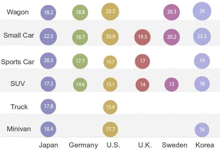
equal number of samples from each country.Visualization
To gain more information regarding countries and cars, we decided to have a visualization of
the data set through the Matrix Chart functionality of the website Many Eyes. In the graph, each
row is a type of vehicle while each column is a country. The average fuel efficiency of a specific
type of car produced in a country is shown and also illustrated with a spherical size on each
grid. The image is below, and we can make these observations from it.
1) Japan leads in the fuel efficiency of sports cars, minivans, and trucks, while ranking
second in that of small cars and SUV's. However, Japan does not produce very fuel-
efficient wagons, ranking the last among six countries.
2) U.S. does very well in fuel efficiency for wagons, in contrast to Japan. It does fairly well
in small cars and SUV's, ranking the third. However, American sports cars are the worst.
3) British vehicles perform badly in all car types.
4) Korean carss are fuel efficient, leading in wagons, small cars, and SUV's. They’re
minivans, however, are not very fuel efficient.Conclusion
After applying various methods on our automobile data set, we can put forth a few conclusions
that follow our analysis results. Due to the limited time and resources, as well as inherent
variations, noises, and uncertainties in our data, much of what we can say remain at a
hypothetical level and we encourage future research in the area.
1) Non-structural factors we analyzed, including country of origin, retail prices and age of
model are mostly not statistically significant in causing a difference in fuel efficiency.
Structural factors, such as weight and horsepower, in contrast, seem to have a strong
impact on fuel economy, with these two examples in particular having a negative relation
with fuel efficiency.
2) Despite this, it is still possible to utilize complex prediction algorithms with non-structural
inputs to obtain a decent prediction of fuel efficiency for a specific vehicle when
combined with the car type variable.Appendix Code 1: Python File Processing
Code 2: Binary Variable Creation
Code 3: SQL Database and Table Creation

sqlite3 FuelEfficiency.db

sqlite3 FuelEfficiency.db
CREATE TABLE Cars(name VARCHAR(50),
                smallCar INTEGER,
                sportsCar INTEGER,
               suv INTEGER,
                wagon INTEGER,
                minivan INTEGER,
                truck INTEGER,
                allWheelDr INTEGER,
                rearWheelDr INTEGER,
                retailPrice INTEGER,
                dealerCost INTEGER,
                engine INTEGER,
                cylinders INTEGER,
              horsepower INTEGER,
                cityFE INTEGER,
                hwyFE INTEGER,
                weight INTEGER,
                wheel INTEGER,
                length INTEGER,
                width INTEGER,
                modelYear INTEGER,
                timePd INTEGER,
              country VARCHAR(10),
                Japan INTEGER,
                Germany INTEGER,
                US INTEGER,
                Korea INTEGER,
                UK INTEGER,
                Sweden INTEGER);

.separator “,”
.import “FuelEfficiency_v3.csv” Cars

Code 4. SQL Queries

SELECT AVG(CityFE), Country
FROM CARS
GROUP BY Country;
Results 1: Country of Car Manufacturer T-tests German-Manufactured Vehicles vs. Non-German Manufactured Vehicles Korean-Manufactured Vehicles vs. Non-Korean Manufactured Vehicles
UK-Manufactured Vehicles vs. Non-UK Manufactured Vehicles

Swedish-Manufactured Vehicles vs. Non-Swedish Manufactured Vehicles
Results 2: Car Type T-tests

SUVs vs. Non-SUVS

Results 3: One-to-One Regressions

Fuel Efficiency vs. Car Length
Fuel Efficiency vs. Car Width

Fuel Efficiency vs. Number of Cylinders
Fuel Efficiency vs. Engine Size
You can also read