Prediction algorithm of fuel mixture in high-altitude cities - Ingenius
←
→
Page content transcription
If your browser does not render page correctly, please read the page content below
Scientific Paper / Artículo Científico
                                                                                    https://doi.org/10.17163/ings.n25.2021.04
                                                                                     pISSN: 1390-650X / eISSN: 1390-860X

               Prediction algorithm of fuel
            consumption for anhydrous ethanol
               mixture in high-altitude cities
           Algoritmo de predicción del consumo
           de combustible para mezcla de etanol
              anhídrido en ciudades de altura
               Fabricio Espinoza1 , Fredy Tacuri1 , Wilmer Contreras1,∗ , Javier Vázquez1

                     Received: 15-05-2020, Reviewed: 05-08-2020, Accepted after review: 30-09-2020

 Abstract                                                      Resumen
 In the present research work, a mathematical model En la presente investigación se obtiene un modelo
 is obtained for predicting specific fuel consumption in matemático de predicción del consumo específico de
 a 1.4-liter Otto cycle engine with electronic injection combustible en un motor ciclo Otto de 1,4 litros
 without making modifications, when using as fuel con inyección electrónica sin hacer modificaciones,
 gasoline mixtures with concentrations in volume of al usar como combustible mezclas de gasolina con
 0%, 25%, 50%, 75% and 100% of anhydrous ethanol. concentraciones a partir de 0 %, 25 %, 50 %, 75 % y
 For the analysis of results, a simplex lattice reticular 100 % en volumen de etanol anhidro. Para el análisis
 mixture experiment design was carried out, which de los resultados se realizó un diseño de experimento
 was subject to an urban driving cycle in the city of de mezcla reticular simplex lattice, el cual se sometió a
 Cuenca at 2558 m above sea level in a roller power un ciclo de conducción urbano de la ciudad de Cuenca
 bank. The data acquisition and the development of a 2558 m s. n. m., en un banco de potencia de rodillos.
 the algorithm were carried out through an analysis of La adquisición de datos y la obtención del algoritmo
 descriptive statistical methods. The validation of the fueron a través de un análisis de métodos estadísticos
 algorithm was performed through residual analysis. descriptivos. La validación del algoritmo se realizó
 As a main result, there is a mathematical model that por medio del análisis de residuos. Como resultado
 enables predicting the engine fuel consumption, for principal se cuenta con un modelo matemático, el
 ranges of ethanol concentration from 0% to 100% in que permite predecir el consumo de combustible del
 the gasoline without needing to conduct real tests.      motor, para rangos de concentración de etanol del
                                                          0 % al 100 % en la gasolina sin la necesidad de realizar
                                                          pruebas reales.
 Keywords: Ethanol anhydride; explanatory model;               Palabras clave: etanol anhídrido, modelo explica-
 fuel consumption                                              tivo, consumo combustible

1,∗
      Universidad Politécnica Salesiana, Cuenca-Ecuador. Corresponding author ): rcontreras@ups.edu.ec.
        http://orcid.org/0000-0003-4559-4474     http://orcid.org/0000-0002-4160-2898
        http://orcid.org/0000-0003-2300-9457     http://orcid.org/0000-0001-9678-5364
Suggested citation: Espinoza, F.; Tacuri, F.; Contreras, W. and Vásquez, J. (2021). «Prediction algorithm of fuel
consumption for anhydrous ethanol mixture in high-altitude cities». Ingenius. N.◦ 25, (january-june). pp. 41-49. doi:
https://doi.org/10.17163/ings.n25.2021.04.

                                                          41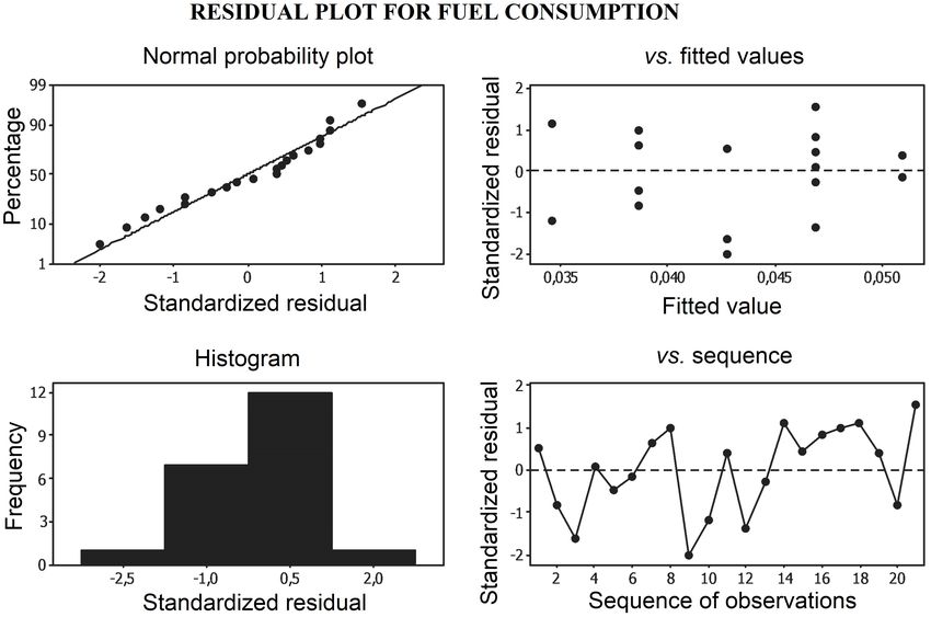
42                                                                        INGENIUS N.◦ 25, january-june of 2021

1. Introduction                                             clude that consumption increases as the concentration
                                                            degree of ethanol in the gasoline increases.
The concern about environmental pollution due to                These research works do not consider in their
residues of incomplete combustion and the depletion         methodology, the development of an experimental de-
of fossil fuels, motivates the study about the refor-       sign by mixtures together with the application of a
mulation of mixtures with alternative fuels. A viable       driving cycle typical of high-altitude cities.
option is applying combinations of ethanol and gaso-            This work was conducted with the purpose of ob-
line, which may reduce air pollution and at the same        taining a mathematical algorithm that enables calcu-
time improve the performance of the motor compared          lating the specific fuel consumption of a Hyundai Getz
with the unmixed oil fuel.                                  1.4-liter vehicle, for different mixtures of anhydrous
     When evaluating the effect of these mixtures, there    ethanol and gasoline at a height of about 2558 meters
is a variation in the total consumption of fuel, in this    above sea level.
line of study, according to the work by Al-Hasan,
(2003) [1]. In a Toyota Tercel vehicle with a four-
                                                            2. Materials and methods
cylinder engine of 1.4 l capacity, four-stroke spark
ignition, compression ratio of 9:1, and a maximum           The methodology applied consists of a simplex retic-
power of 52 kW at 5600 rpm, results in an approximate       ular (q, m) experimental design by mixtures, which
increase of 8.3%, 9%, 7% and 5.7% in fuel consumption.      considers q components and enables fitting a statis-
     When biofuels are used in internal combustion en-      tical model of order (m); this consists of all possible
gines, consumption of such fuels increase [2]. This is      combinations of components or mixtures that may
due to the fact that if the air-fuel stoichiometric ratio   be formed considering that proportions may take the
decreases for the same revolutions per minute, same         (m+1) values between zero and one, given by Equation
load level and same air mass, the required fuel mass        1 [22].
should be greater [3].
     Fernández, Mosquera, and Mosquera [4] demon-                                  0.1 0.2        m
                                                                               xi =   ,    ,...,                  (1)
strated that the use of ethanol mixed with gasoline                                 m m           m
increases the consumption linearly with the mixture             The anhydrous ethanol-gasoline mixture is identi-
used.                                                       fied with the nomenclature (E) followed by a number,
     In the research conducted in a Lada vehicle with       the letter represents the mixture, and the number indi-
a 1.3 l four-stroke engine and a carburation feeding        cates the percentage of ethanol added to the gasoline.
system, the fuel used is a 10, 20 and 30% mixture of        This mixture is characterized by its density, which
anhydrous ethanol in regular gasoline, of which Melo        is obtained using the method of the pycnometer, the
et al. [5] conclude that as the percentage of ethanol in    octane rating by means of an octane rating meter that
the mixture increases, fuel consumption increases for       meets the ASTM 2699 – 86 standard, and the high
all the evaluated experimental points.                      and low calorific value (HH cs Ex ), (H
                                                                                                  H ci Ex ) according
     In the study conducted by Delión and Rojas [6] in a    to Equations 2 and 3, that enable calculating this
1.4 liter Ford vehicle with respect to fuel consumption     property [23].
for ethanol and gasoline mixtures, it was found that
the «increase of fuel consumption is greater due to the
                                                             H cs   Ex      E × H Cs
                                                                         = %E          etanol   + %G × H Cs   gasolina   (2)
increase in load or motor torque, maintaining the rpm
constant, and the polluting emissions are lesser than
with pure gasoline».
     On the other hand, studies conducted in 1997, 1998      H ci   Ex      E × H Ci
                                                                         = %E          etanol   + %G × H Ci   gasolina   (3)
and 1999 by Kortum et al. [7], Apace [8] and Ragazzi            In order to obtain the mathematical model, the
and Nelson [9], respectively, match the research studies    data are statistically validated using the test for out-
carried out in 2003 by Al-Hassan [1], He et al. [10] and    liers, and a statistical model is fitted to investigate
Patzek [11], 2004 by Wu et al. [12], 2005 by Coelho et      the effect of the components on the response. A first
al. [13], Hansen et al., Niven [14] and American Coali-     approximation may be obtained fitting a first order
tion for Ethanol [15], 2006 by Behrentz [16], Durbin        model (Equation 4).
et al. [17], Shapiro [18] and Yucesu et al. [19], 2008 by
Acevedo et al. [20], as well as the more recent works                                      q−1
                                                                                           X
by Doe et al. [21], in which fuel consumption increases                          E(y) =          βi χi                   (4)
from 1 to 6% in engines without modification using                                         i=1
mixtures with 0-25% of ethanol, since the consumption           When fitting a quadratic model, it is also necessary
depends on the electronic control system of the engine.     to incorporate the constraint x1 + x2 + . . . + xq = 1,
     Research works conducted about fuel consumption        because this will give a special characteristic to the
for mixtures of anhydrous ethanol and gasoline, con-        model. To illustrate the idea, it is assumed that there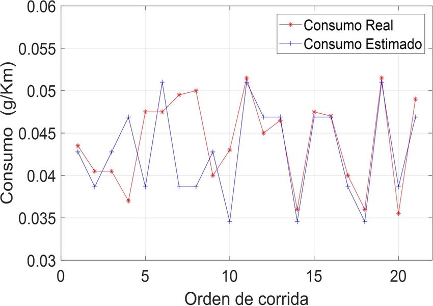
Espinoza et al. / Prediction algorithm of fuel consumption for anhydrous ethanol mixture in high-altitude
cities                                                                                                                     43

are three components, x1, x2, x3, and thus the second
order polynomial is given by Equation 5.                                           q                q
                                                                                   X               XX
                                                                          E(y) =         βi χi +             βij χi χj +
                                                                                   i=1             i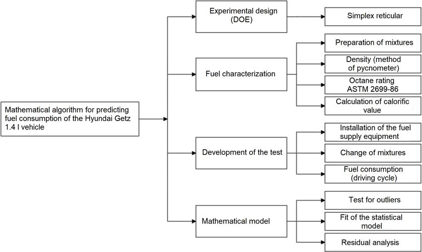
44                                                                    INGENIUS N.◦ 25, january-june of 2021

                                       Table 1. Random experimental design

          Sequence established     Run sequence      Type Pt.     Blocks       ETHANOL        GASOLINE
                    17                     1                0        1            0,5               0,5
                    16                     2                2        1           0,25              0,75
                    3                      3                0        1            0,5               0,5
                    14                     4               –1        1           0,75              0,25
                    9                      5                2        1           0,25              0,75
                    19                     6                1        1             1                 0
                    2                      7                2        1           0,25              0,75
                    13                     8               -1        1           0,25              0,75
                    10                     9                0        1            0,5               0,5
                    1                     10                1        1             0                 1
                    12                    11                1        1             1                 0
                    21                    12               –1        1           0,75              0,25
                    7                     13               –1        1           0,75              0,25
                    15                    14                1        1             0                 1
                    11                    15                2        1           0,75              0,25
                    18                    16                2        1           0,75              0,25
                    20                    17               –1        1           0,25              0,75
                    8                     18                1        1             0                 1
                    5                     19                1        1             1                 0
                    6                     20               –1        1           0,25              0,75
                    4                     21                2        1           0,75              0,25

                               Table 2. Physicochemical properties of the mixtures

                                               Physicochemical properties
                 Fuel                          Octane rating    High calorific     Low calorific
                         Density (kg/m3 )
                                                  (RON)         value (kJ/kg)      value (kJ/kg)
                  E0            740                 85,6            47   300            44   000
                 E25            760                90,95            42   900            39   725
                 E50           768,7               96,3             38   500            35   450
                 E75            782               101,65            34   100            31   175
                 E100          790,7                107             29   700            26   900

2.3. Measurement of fuel consumption                        equipment in the vehicle; Table 3 indicates the data
                                                            obtained according to the design of experiment
This research is developed in the city of Cuenca
(Ecuador) located at 2558 meters above sea level, the
fuel consumption tests are carried out in a 1.4-liter
Hyundai Getz vehicle with electronic injection sys-
tem and treatment of gases with a three-way catalytic
converter; the compression ratio is 9,5:1, DOHC dis-
tribution system with four valves per cylinder and
atmospheric type aspiration Hyundai Motor Company
(2011) [26].
    For performing the different tests of this research
work, the original fuel feeding system of the vehicle is
replaced by an alternate supply system meeting the
technical specifications of the manufacturer, with the
purpose of preventing alterations in the fuel mixtures.
    The equipment utilized for measuring fuel con-
sumption is the FLOW-MASTER MAHA CH-4123
flow meter. Figure 2 illustrates the installation of the                 Figure 2. Tests of operation 1
Espinoza et al. / Prediction algorithm of fuel consumption for anhydrous ethanol mixture in high-altitude
cities 45
Table 3. Measurement of fuel consumption
Fuel
Sequence established Run sequence ETHANOL GASOLINE consumption (g/km)
17 1 0,5 0,5 0,0435
16 2 0,25 0,75 0,0405
3 3 0,5 0,5 0,0405
14 4 0,75 0,25 0,037
9 5 0,25 0,75 0,0475
19 6 1 0 0,0475
2 7 0,25 0,75 0,0495
13 8 0,25 0,75 0,05
10 9 0,5 0,5 0,04
1 10 0 1 0,043
12 11 1 0 0,0515
21 12 0,75 0,25 0,045
7 13 0,75 0,25 0,0465
15 14 0 1 0,036
11 15 0,75 0,25 0,0475
18 16 0,75 0,25 0,047
20 17 0,25 0,75 0,04
8 18 0 1 0,036
5 19 1 0 0,0515
6 20 0,25 0,75 0,0355
4 21 0,75 0,25 0,049
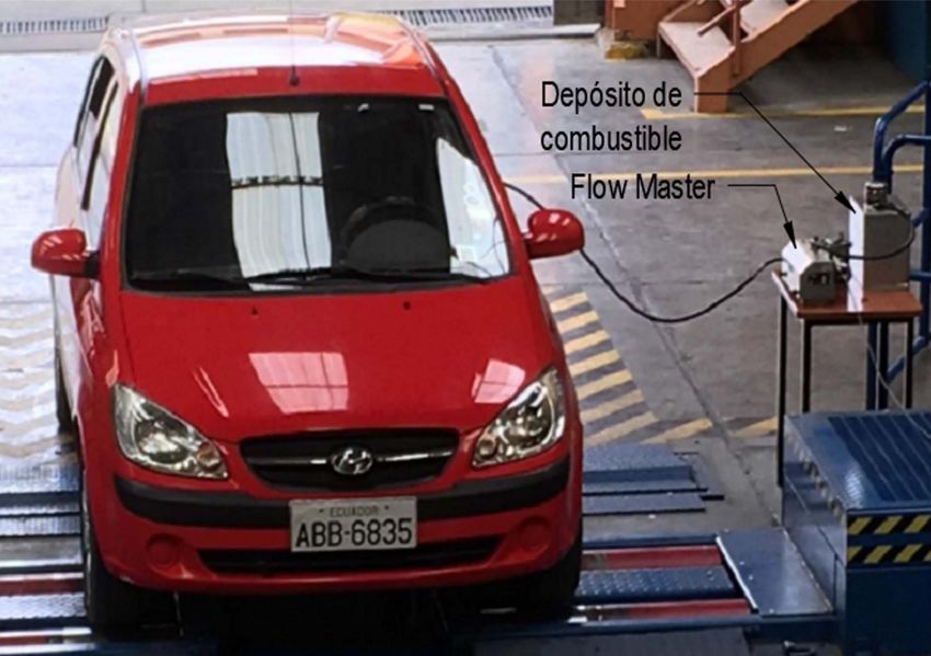
To obtain specific fuel consumption, it was utilized most distinctive ones as determined by means of a
the driving cycle representative of the city of Cuenca, pre-experimental analysis. The test is carried out on a
which is identified in Figure 3; a micro-cycle is ap- Maha LPS 3000 power bank.
plied with the first five minutes, since they are the
Figure 3. Driving cycle representative of the city of Cuenca
2.4. Data treatment for the response model After the data have been validated the model is con-
structed, and a residual analysis is performed with
With the data of the experimental design as a function the purpose of verifying the hypotheses of normality,
of the different mixtures, it is convenient to conduct homoscedasticity, independence and linearity of the
validation tests of the results before proceeding to model.
obtain the response model. The R22 Dixon test for
outliers [27] was established for validating the results.46 INGENIUS N.◦ 25, january-june of 2021
3. Results and discussion models are greater than the 0.05 significance level, and
thus these models are not considered.
In order to determine the model that explains fuel
After the linear model has been selected, the es-
consumption, a multivariable linear regression analysis
timated regression coefficients are determined (Table
is carried out with the data obtained from the DOE,
5), and it is obtained the formula of the model for
and a higher order model is fitted as indicated in Table
predicting consumption shown in Equation 7.
4, where the different values of «R2» and «p-value»
are observed. This information enables choosing the
linear model, to meet the assumptions, and it is also
observed in the «p-value» column that the higher order 2Y = 0.05100(etanol) + 0, 03455(gasolina) (7)
Table 4. Summary of the models fitted for fuel consumption
Model P-value (%) Predicted (%) Adjusted (%)
Linear 0 94,2 93,04 93,86
Quadratic 0,274 94,6 92,66 93,94
Complete cubic 0,784 94,6 91,92 93,62
Complete cubic 0,126 95,3 91,59 94,17
Note. Value *p < 0,05
Table 5. Regression coefficients estimated for fuel consumption
Term Coeff. EE of the coeff. T P VIF
ETHANOL 0,051 0,000562 * * 1,19
GASOLINE 0,03455 0,000562 * * 1,19
Note. Value *p < 0,05
The results indicated in Figure 4 are obtained after been conducted, graphical results are shown in the
applying Equation 7. following which confirm the fit of the model to the fuel
In addition, in the variance analysis for the linear consumption.
model, as indicated in Table 6, the «p-value» = 0,000,
therefore, the model is significant and with a very good In order to evaluate the model of fuel consumption,
adjusted «R2 » of 93.86. a four in one residuals plot is utilized, as indicated in
The remaining models are excluded because they Figure 5. This graphical analysis with respect to the
do not meet the p-value assumption [28]. standardized residuals, enables verifying the fit of the
Once the standardized analysis of variance has experimental model obtained previously.
Figure 4. Result of the numerical algorithmEspinoza et al. / Prediction algorithm of fuel consumption for anhydrous ethanol mixture in high-altitude
cities 47
Table 6. Variance analysis for fuel consumption
Source GL SC Sec. SC Adjust. MC Adjust. F P
Regression 1 0,00061 0,000609 0,000609 306,5 0
Linear 1 0,00061 0,000609 0,000609 306,5 0
Residual error 19 3,8E-05 0,000038 0,000002
Lack of adjustment 3 8E-06 0,000008 0,000003 1,34 0,3
Pure error 16 0,00003 0,00003 0,000002
Total 20 0,00065
Note. Value *p < 0,05
Figure 5. Residuals plots for the fuel consumption data
From the analysis of Figure 5, the following con- random pattern around the central line, no as-
clusions are drawn: cending or descending trends of the observations
occur that indicate a bad fit of the model.
a. The normal probability plot shows that the resid-
uals follow a normal distribution, since the fit to With this analysis it is concluded that the variance
a normal trend line. is correct and that the model does not exhibit anoma-
lies in the results, and thus it may be used to predict
b. The Histogram plot of the residuals is bell- fuel consumption in a better manner.
shaped, having a value of –2,02 for observation
Figure 6 shows a plot of the response of the mix-
number nine, which is out of the allowed range
ture (ethanol-gasoline) in the fuel consumption. This
(–2,0) in standard residual; however, this does
enables evaluating how the components are related to
not have a greater significance in the model, and
the response using a fitted model.
the normality of the data is accepted.
The tracking plot of fuel consumption shown in
c. On the other hand, in the plot of standard- Figure 6, provides the following information about the
ized residuals versus fitted values, no abnormal effects of the components:
trend is observed that indicates a bad fit of It is observed that fuel consumption has a growing
the model, since the residuals are randomly dis- trend as the ethanol increases up to a maximum in
tributed around zero, and thus it is considered E100, while decreases the concentration of the second
that there is independence. component, in this case gasoline extra.
Also note that the slope of the curve is steeper in
d. At last, in the plot of standardized residuals the section between 0 and 15% of ethanol, and in the
versus the sequence of observations, there is a section after 40%; therefore, in the range between 1548 INGENIUS N.◦ 25, january-june of 2021
and 40% it is less step, corresponding to the zone of [3] CEPAL, “Consideraciones ambientales en torno
less fuel consumption. a los biocombustibles líquidos,” in División de
Desarrollo Sostenible y Asentamientos Humanos,,
2008.
[4] S. Fernández Henao, J. Mosquera A., and
J. Mosquera M., “Análisis de emisiones de CO2
para diferentes combustibles en la población de
taxis en Pereira y Dosquebradas,” Scientia et
Technica, vol. 2, no. 45, ago. 2010. [Online].
Available: https://doi.org/10.22517/23447214.385
[5] E. A. Melo Espinosa, Y. Sánchez Borroto,
N. Ferrer Frontela, and N. Ferrer Frontela,
“Evaluación de un motor de encendido por
chispa trabajando con mezclas etanol-gasolina,”
Ingeniería Energética, vol. 33, pp. 94–102, 08 2012.
[Online]. Available: https://bit.ly/38kOxFW
[6] J. Goñi Delión and M. Rojas-Delgado, “Com-
Figure 6. Tracking plot of fuel consumption response bustibles alternativos en motores de combustión
interna,” Ingeniería Industrial, 02 2014. [Online].
Available: https://doi.org/10.26439/ing.ind2014.
n032.122
4. Conclusions and recommendations
[7] J. Gibbons, Interagency Assessment of Oxy-
Specific fuel consumption is directly proportional to genated Fuels. National Science and Tech-
the percentage of ethanol in the mixture, i.e., as the nology Council, 1997. [Online]. Available:
percentage of ethanol in the mixtures increases, spe- https://bit.ly/355W21N
cific fuel consumption increases as well. Therefore,
with an E20 mixture there is a 7% increase in fuel [8] Apace Research Ltd, “Intensive field trial of
consumption, while in an E100 mixture there is 31.3% ethanol/petrol blend in vehicles,” ERDC Project
more consumption with respect to the gasoline of 86.5 No. 2511, Tech. Rep., 1998. [Online]. Available:
octanes. https://bit.ly/32iZaFK
It was established a mathematical model that en- [9] R. Ragazzi and K. Nelson, “The impacts of a
ables determining fuel consumption for different per- 10 % ethanol blended fuel on the exhaust emis-
centages of ethanol in the gasoline, which can be ap- sions of tier 0 andtier 1 light duty gasoline vehicles
plied for contrasting real tests. al 35 f,” Colorado Department of Public Health
The increase in fuel consumption is due to the re- and Environment, 1999.
duction of the calorific value of the mixture as the
concentration of ethanol varies. [10] B.-Q. He, Jian-Xin Wang, J.-M. Hao, X.-G. Yan,
During the development of the tests, the vehicle and J.-H. Xiao, “A study on emission charac-
operated correctly without showing anomalies for con- teristics of an efi engine with ethanol blended
centrations greater than 30%. gasoline fuels,” Atmospheric Environment, vol. 37,
no. 7, pp. 949–957, 2003. [Online]. Available:
https://doi.org/10.1016/S1352-2310(02)00973-1
References
[11] T. W. Patzek, S.-M. Anti, R. Campos, K. W. ha,
[1] M. Al-Hasan, “Effect of ethanol–unleaded J. Lee, B. Li, J. Padnick, and S.-A. Yee, “Ethanol
gasoline blends on engine performance from corn: Clean renewable fuel for the future,
and exhaust emission,” Energy Conver- or drain on our resources and pockets?” Envi-
sion and Management, vol. 44, no. 9, ronment, Development and Sustainability, vol. 7,
pp. 1547–1561, 2003. [Online]. Available: no. 3, pp. 319–336, Sep. 2005. [Online]. Available:
https://doi.org/10.1016/S0196-8904(02)00166-8 https://doi.org/10.1007/s10668-004-7317-4
[2] H. L. MacLean and L. B. Lave, “Evaluating [12] C.-W. Wu, R.-H. Chen, J.-Y. Pu, and T.-H.
automobile fuel/propulsion system technologies,” Lin, “The influence of air-fuel ratio on engine
Progress in Energy and Combustion Science, performance and pollutant emission of an si
vol. 29, no. 1, pp. 1–69, 2003. [Online]. Available: engine using ethanol-gasoline-blended fuels,” At-
https://doi.org/10.1016/S0360-1285(02)00032-1 mospheric Environment, vol. 38, no. 40, pp.Espinoza et al. / Prediction algorithm of fuel consumption for anhydrous ethanol mixture in high-altitude
cities 49
7093–7100, 2004, 8th International Conference [20] H. R. Acevedo G. and J. M. Mantilla G.,
on Atmospheric Sciences and Applicat ions “Viabilidad ambiental del uso de biocombustibles
to Air Quality (ASAAQ). [Online]. Available: para motores a gasolina y diésel en colombia,”
https://doi.org/10.1016/j.atmosenv.2004.01.058 Boletin del Observatorio Colombiano de Energía,
Bogota. D. C., pp. 3–14, 2008. [Online]. Available:
[13] S. T. Coelho, J. Goldemberg, O. Lucon, and https://bit.ly/38kSXg0
P. Guardabassi, “Brazilian sugarcane ethanol:
lessons learned,” Energy for Sustainable Develop- [21] U.S. Department of Energy, “Handbook for
ment, vol. 10, no. 2, pp. 26–39, 2006. [Online]. handling, storing, and dispensing e85 and other
Available: https://bit.ly/2JJIeBM ethanol-gasoline blends,” U.S. Department of
Energy, Tech. Rep., 2013. [Online]. Available:
[14] R. K. Niven, “Ethanol in gasoline: environmental https://bit.ly/2U1zVmF
impacts and sustainability review article,” Re-
[22] H. Gutiérrez Pulido and R. de la Vara Salazar,
newable and Sustainable Energy Reviews, vol. 9,
Análisis y diseño de experimentos. McGraw-Hill,
no. 6, pp. 535–555, 2005. [Online]. Available:
2003. [Online]. Available: https://bit.ly/36gB7rU
https://doi.org/10.1016/j.rser.2004.06.003
[23] E. A. García, “Modelización termodinámica
[15] American Coalition For Ethanol. (2005) Fuel de un motor turboalimentado y propul-
economy study: comparing performance and sado por bioetano,” 2009. [Online]. Available:
costs of va-rious ethanol blends and stan- https://bit.ly/3k85tBO
dard unleaded gasoline. [Online]. Available:
https://bit.ly/32mEmwP [24] INEN, “NTE INEN 2478: Etanol anhidro.
requisitos,” Instituto Ecuatoriano de Normali-
[16] E. Behrentz, Beneficios ambientales asociados zación, Tech. Rep., 2009. [Online]. Available:
con el uso de combustibles alternativos. Cen- https://bit.ly/354abwc
tro de Investigaciones en Ingeniería Ambiental
(CIIA) Universidad de los Andes, 2008. [Online]. [25] ——, “NTE INEN, Gasolina. Requisitos,” Insti-
Available: https://bit.ly/38k6cOj tuto Ecuatoriano de Normalización, Tech. Rep.,
2012. [Online]. Available: https://bit.ly/2JLGsQD
[17] T. Durbin, J. W. Miller, T. Huai, D. R.
[26] Hyundai. (2011) Manual del taller. [Online].
Cocker III, and Y. Younglove, “Effects of ethanol
Available: https://bit.ly/356tPIc
and volatility parameters on exhaust emissions of
light-duty vehicles.” in UC Riverside: Center for [27] S. P. Verma and A. Quiroz-Ruiz, “Critical values
Environmental Research and Technology. [Online]. for six Dixon tests for outliers in normal samples
Available: https://bit.ly/3oZFmkp up to sizes 100, and applications in science
and engineering,” Revista Mexicana de Ciencias
[18] E. Shapiro. (2006) Roundtable on ethanol fuel: Geológicas, vol. 23, pp. 133–161, 01 2006. [Online].
automaker view. Available: https://bit.ly/3eBoOKG
[19] H. S. Yücesu, T. Topgül, C. Çinar, and M. Okur, [28] W. Contreras, J. Ortega, and R. Japa, “Aplicación
“Effect of ethanol-gasoline blends on engine de una red neuronal feed-forward backpropa-
performance and exhaust emissions in different gation para el diagnóstico de fallas mecánicas
compression ratios,” Applied Thermal Engineer- en motores de encendido provocado,” INGE-
ing, vol. 26, no. 17, 2006. [Online]. Available: https: NIUS, pp. 32–40, 2019. [Online]. Available:
//doi.org/10.1016/j.applthermaleng.2006.03.006 https://doi.org/10.17163/ings.n21.2019.03You can also read