Letting the machines do the maths: an AI predicting cryptocurrency movements - UCL
←
→
Page content transcription
If your browser does not render page correctly, please read the page content below
Letting the machines do the maths: an AI predicting
                    cryptocurrency movements
                                     Cezary Klimczuk
                      1
                          BSc Economics, University College London

1. Introduction
        Since the invention of the biggest cryptocurrency - Bitcoin (BTC) - in 2008, there
has been a rising interest in the cryptocurrency market, as well as blockchain technology.
Cryptocurrencies are decentralized digital assets, serving as a medium of exchange.
Its decentralized nature comes from the distributed ledger technology based on strong
cryptography and a proof-of-work technique (Nakamoto, 2009). In February 2020, the
cryptocurrency market capitalization reached $292.2bn (CoinMarketCap, 2020). This
figure is higher than the nominal GDP of countries like New Zealand, Qatar or Ukraine;
and is predicted to raise in the near time horizon (Global Cryptocurrency Market, 2019).

For many, this technology is seen as a solution to the intermediary problem, others
perceive cryptocurrencies as extremely volatile assets capable of bringing over-the-
market-rate margins. (Conrad et al., 2018) has shown that cryptocurrency markets - the
market for bitcoin in particular - demonstrate very high levels of volatility in comparison
to commodities, stocks or traditional currency markets. It is also very weakly correlated
with other markets.

The most natural choice for time-series data, autoregression models, have been
shown by (Abu Bakar et al., 2017) and (Adebiyi et al., 2014) to produce high error
margins, hence being not the most efficient tool in predicting future price movements.
As predicting future price movements seems to be a non-linear task, artificial neural
networks started to become more popular in modelling the stock market.

This paper firstly introduces the idea of Neural Networks and describes its features
allowing it to be a particularly handy tool for this type of task. Then I move onto
reviewing literature concerning some of the approaches used by other scholars to predict
future cryptocurrency prices. Lastly, I present my own Neural Network architecture and
asses its performance based on a redefined evaluation metric not yet encountered in any
of the papers concerning this topic.

2. Artificial Neural Networks (ANN)
        ANNs are biologically inspired structures, resembling to a large extent the process
taking place in living organisms’ brains. Similar to our brains, neural networks consist
of layers of nodes, which aim to model neurons in a living organism. Figure 1 shows a
basic example of a network with 4 inputs, which values are further passed to next layers.
The value reaching a red node is a weighted sum of the 4 input nodes A, B, C, D. Bear in
mind, these weights can be different for each node. The same process is applied to green
(weighted sum of red nodes) and then blue nodes up until we calculate the final output.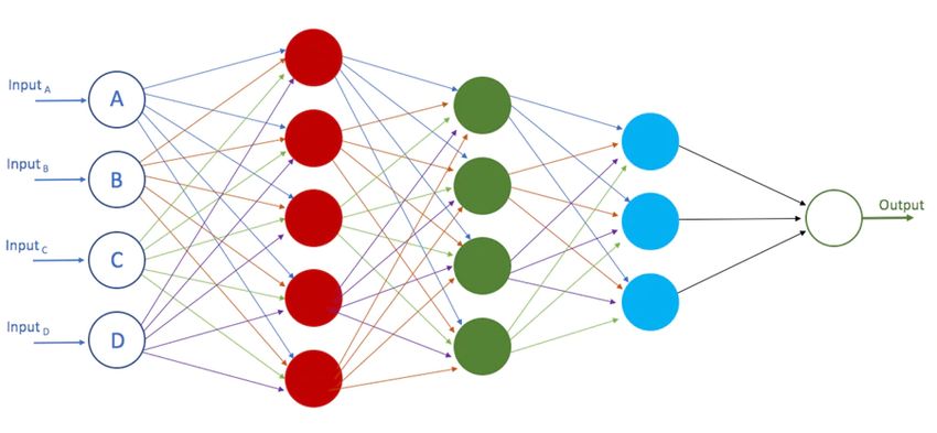
Figure 1. An example of a dense neural network

We can see that the connections between the nodes, ANN links, are responsible for
transferring signals from layer to layer, much like axons do in a human brain. The
weighted sum of those connections constitutes the aggregate signal passed to the next
neuron.

However, the signal reaching a neuron must be strong enough to be transferred
further. To ensure that, we use an activation function, which in simple terms asks: ”Is
the signal strong enough?” If yes, then pass the signal. That process is shown in the
right bottom corner of Figure 2. This introduces non-linearity to the model and allows it
to recognize more complex patterns than more traditional machine learning techniques
(Kustrin et al., 2000). There is a wide range of activation functions that we can use as
shown by (Czekalski et al., 2015).

       Figure 2. A comparison between biological and digital neuron architecture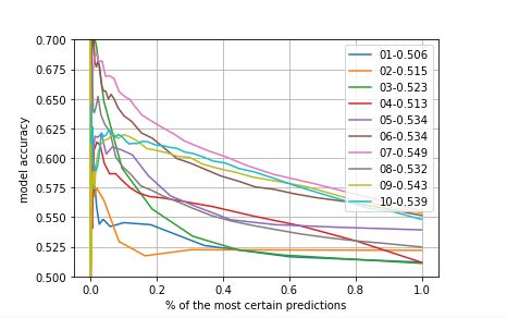
The ANN is initialized with random weights. What makes ANNs so powerful, is their
ability to improve weights over time. This is done by checking the error of the final
output, i.e. how far away the network was from the “true” value, and then updating the
weights to reduce that error (defined in variety of ways dependent on the type of problem
we are solving). During this process some connections are strengthened, and some
are weakened, so that the network produces smaller error next time. After evaluating
thousands of examples, the neural network learns how to detect certain patterns and
yields accurate results. There are many different techniques of updating these weights, of
which the most popular one is the backpropagation algorithm. Once the network satisfies
sufficient benchmarks on the test set, the updated links are saved and then used to predict
future outcomes (Balaji et al., 2013)

There is a variety of neural network types characterized by some very technical
differences. One type, that will be of our interest in this paper, is the Recurrent Neural
Network (RNN). It is a specific class of neural networks able to make use of sequential
data – a type of data, where the order of occurrence matters. (Sak et al., 2014) showed
this is particularly useful in the field of Natural Language Processing, as human speech
is a sequenced type of data, where the meaning of a word depends on words preceding it.

The hope is that this type of architecture would be useful for our price movement
prediction task and will learn dynamic patterns from the sequential nature of trading data.

3. Literature study
        Researchers tried to compare basic average-based models (e.g. ARIMA) with
dense neural networks – similar to the one shown in Figure 1. (Munim et al., 2019)
compared the two by evaluating the accuracy using the Mean Absolute Percentage Error.
They simply asked: “What is the difference between the predicted price of bitcoin the
day before of each model and the true price?”. The study was concluded using training
dataset of 2000 days of bitcoin trading. Despite the dense neural network complexity,
ARIMA model turned out to yield smaller errors for all measurement techniques. This
study showed that dense networks do not perform well in a time-series setting.

On the contrary, (McNally et al., 2018) arrived at different results by using slightly
modified architectures, namely Bayesian optimized recurrent neural network (RNN)
and a Long Short Term Memory (LSTM) network versus the ARIMA model. Unlike
in the previous study, the model output was designed to indicate whether the price of
bitcoin will go up or down the next day (not to predict the exact value). The ARIMA
model gave the correct prediction only 50.05% of times. Both RNN and LSTM scored
better – 50.25% and 52.78% respectively. This research showed the benefit of using
recurrent-based type architectures in forecasting tasks.

(Radityo et al., 2017) study focused more on exploring learning techniques i.e.
ways in which the weights in the network are updated. They used 4 main learning
techniques: BPNN, GANN, GABPNN, and NEAT. They evaluated the performance of
these models, using mean average percentage error (MAPE), similarly to the previous
study (Munim et al., 2019).
Learning technique Mean Absolute Percentage Error
Backpropagation Neural Network 1.998%
(BPNN)
Genetic Algorithm Neural Network 4.461%
(GANN)
Genetic Algorithm Backpropagation 1.883%
Neural Network (GABPNN)
Neuroevolution of augmenting topologies 2.175%
(NEAT).
Interestingly enough, GANN performed better in the case of stock market (Nayak
et al., 2012). This shows there is a fundamental difference in these both markets linked
to the volatility of cryptocurrencies. These findings indicate that our model should lean
towards backpropagation-based techniques.
4. The model
One conclusion we can immediately draw from above findings is the inconsis-
tency of performance metrics. Some papers evaluate models by looking at the percentage
error of the predicted value, like (Munim et al., 2019), others try to optimize for correct
up/down prediction as in (McNally et al., 2018). Before constructing our model, we need
to decide what do we want to optimize for, to make our model useful.
Most traders, while making the decision whether to buy or not, tend to ask them-
selves “Do I think the price is going to go up or down?”. Then based on their intuition
and experience they make the decision. However, their performance is not evaluated
based on how many times they were “right”, rather it is assessed by the rate of return
yielded by their portfolio. Hence, I decided that my model will learn how to invest
similarly to (McNally et al., 2018), but I will test its performance by letting it trade over
the test period.
4.1. Data
Unlike in aforementioned research papers, I am using minute-by-minute market
data instead of day-by-day. It consists of Ethereum and Bitcoin prices from 2018 and
2019. The data inputs involve values of open and close prices, maxima and minima and
trading volumes on any given minute. The data is then split into training and validation
sets, but only the 2018 part. The prices of 2019 are left solely to test the model’s behaviour
evaluated over a sample further apart in time.
4.2. Architecture
The input to the neural network consists of 45 minutes worth of trading data de-
scribed above and the network tries to predict an upward or downward movement of
Ethereum price within the next 3 minutes. The output is a probability distribution. If the
probability for up is > 50%, then up is predicted and vice versa. Following up on the
on the findings of (McNally et al., 2018) and (Radityo et al., 2017) I experimented with
various mixtures of LSTM and dense layers of the neural networks. In general, all of the
architectures were yielding similar results with slight tendency of accuracy falling whenincreasing the complexity of the model. The network learned through the backpropaga-
tion algorithm and returned adjusted probabilities of upward or downward movement. I
trained the model through 10 epochs, which means I performed the training operation
using the entire training set 10 times. After each time, I saved the model from that pass.
4.3. Results
All architectures have been trained only through 10 epochs, as further learning
suffered from a significant overfitting (i.e. remembering the results rather than learning
patterns). The best model was able to indicate the correct direction of price change on
54.9% of instances. However, this is not the whole story. Some predictions are more
“certain” than others. Recall that the network predicts up when the probability of up is
bigger than 50%. Now, that is true for both scenarios where the probability is 50.01% as
well as 60%.
I wanted to see, if the accuracy would increase if we took only relatively “certain”
predictions made by the network. To do so, I plotted the prediction accuracy of each
model (y axis) versus the ratio of the most “certain” predictions (x axis). As we can
see in Figure 3, the more certain predictions we take, the better results it yields. For
instance, the best preforming model “07-0.549” has 54.9% accuracy when evaluated over
the entire validation set, however the percentage of correct predictions grows way above
62.5% for the 20% of the most certain indications.
Figure 3. Models’ accuracy versus % of most certain predictions
This shows that decisions made by the network have some underlying logic embedded in
historical patterns. Those patterns – however complex they could be – can be extended to
predict future outcomes with certain degree of accuracy.I mentioned at the beginning of this section that I did not want to stop evaluating
my model just by looking at the percentage of correct guesses. Therefore, I let the model
decide whether to buy or sell Ethereum at these short 3-minute interval over the entire
year 2019. I assume no transaction costs, immediate execution of the order and perfect
market liquidity (I can buy or sell as much as I want for the market price). The trading
activity is as follows:
- Consider the last 45 minutes of BTC and ETH price data
- Feed them trough the network and decide whether to buy or sell ETH
- Enter a long/short position based on the network prediction
- After 3 minutes close the position
- Repeat this activity minute-by-minute
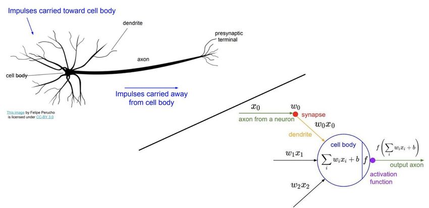
Because there is 24 × 60 minutes in a day, the model makes 1440 trades a day. Each trade
is associated either with a loss or a profit. We can plot the model returns over the trading
time.
Figure 4 shows the daily returns averaged over a sample of 350 trading days. The
green line represents the average of all trading days. We can see, that the average daily
return from the trading activity using the model predictions is 40.7%. That is in line with
theoretical expectations. The standard deviation of ETH return in a 3-minute interval is
0.00275 with expected value of 1. Assuming 55% prediction accuracy, the daily return
should be
(1.002750.55 × 0.997250.45 )1440 = 1.4478 ≈ 44.8%
Figure 4. Average daily returns from the trading activity5. Conclusion
Although these results might suggest that a model like that is capable of bringing
infinite returns, it is important to bear in mind that it has been evaluated only in theoretical
framework, where we do not encounter many limitations associated with trading activity,
which I excluded from the model. These are:
- Bid/ask spread – our model assumed a single value for which we can buy or sell
an infinite amount of the asset at any point in time. The reality is however, that
every exchange has a finite number of orders at any given moment. Therefore,
we cannot buy or sell more than market participants are willing and able to sell or
buy.
- Market capacity – making trades on a relatively small scale won’t impact the mar-
ket behaviour, however as the capacity of the portfolio increases, it might affect
the price by influencing the aggregate market demand/supply.
- Transaction costs – making an order is costly in comparison to the return one can
make from a 3-minute investment. That alone is a big obstacle for implementation
of such model as it might rarely (or never) be the case that investing on such short
timescales brings any returns.
However, what this paper does show, is the fact that short-term cryptocurrency movements
can be successfully modelled thanks to the speculative nature of the market. Because the
value is largely driven by the hope of making a profit and fear of losses (unlike for exam-
ple the FOREX market, where currencies reflect socio-economic events), cryptocurrency
trading demonstrates some characteristics of a game. Assuming that cryptocurrency trad-
ing is an instance of a game theory problem, we can conclude that carefully designed
neural network is capable of outsmarting other market participants.References
[1] Nakamoto, Satoshi. (2009). Bitcoin: A Peer-to-Peer Electronic Cash System.
[2] CoinMarketCap. (2020). Global Charts — CoinMarketCap. [online] Available at:
https://coinmarketcap.com/charts/ [Accessed 11 Feb. 2020].
[3] Global Cryptocurrency Market: Analysis By Type, By Constituents, By Region, By
Country (2019 Edition): Opportunities and Forecast (2017-2024)
[4] Conrad, Christian Custovic, Anessa Ghysels, Eric Lv, Kaia. (2018). Long-and Short-
Term Cryptocurrency Volatility Components: A GARCH-MIDAS Analysis. SSRN
Electronic Journal. 10.2139/ssrn.3161264.
[5] Abu Bakar, Nashirah Rosbi, Sofian. (2017). Autoregressive Integrated Moving Average
(ARIMA) Model for Forecasting Cryptocurrency Exchange Rate in High Volatility
Environment: A New Insight of Bitcoin Transaction. International Journal of Ad-
vanced Engineering Research and Scinece. 4. 10.22161/ijaers.4.11.20.
[6] E. Khan, “Neural fuzzy based intelligent systems and applications,” in Fusion of Neu-
ral Networks, Fuzzy Systems, and Genetic Algorithms Industrial Application, C. J.
Lakhmi and N. M. Martin, Eds., The CRC Press International Series on Computa-
tional Intelligence, pp. 107–139, CRC Press, New York, NY, USA, 2000.
[7] Kustrin, Snezana Beresford, Rosemary. (2000). Basic concepts of artificial neu-
ral network (ANN) modeling and its application in pharmaceutical research.
Journal of pharmaceutical and biomedical analysis. 22. 717-27. 10.1016/S0731-
7085(99)00272-1.
[8] Czekalski, Piotr Niezabitowski, Michał Stybliński, Rafał. (2015). ANN for FOREX
Forecasting and Trading. 10.1109/CSCS.2015.51.
[9] Balaji, S. Baskaran, K.. (2013). Design and Development of Artificial Neural Network-
ing (ANN) System Using Sigmoid Activation Function to Predict Annual Rice Pro-
duction in Tamilnadu. International Journal of Computer Science, Engineering and
Information Technology. 3. 10.5121/ijcseit.2013.3102.
[10] Sak, Haşim Senior, Andrew Beaufays, Françoise. (2014). Long Short-Term Mem-
ory Based Recurrent Neural Network Architectures for Large Vocabulary Speech
Recognition.
[11] Munim, Ziaul Shakil, Mohammad Alon, Ilan. (2019). Next-Day Bitcoin Price Forecast.
Journal of Risk and Financial Management. 12. 10.3390/jrfm12020103.
[12] McNally, Sean Roche, Jason Caton, Simon. (2018). Predicting the Price of Bitcoin Using
Machine Learning. 339-343. 10.1109/PDP2018.2018.00060.
[13] Radityo, Arief Munajat, Qorib Budi, Indra. (2017). Prediction of Bitcoin exchange rate to
American dollar using artificial neural network methods. 433-438. 10.1109/ICAC-
SIS.2017.8355070.
[14] Nayak, Sarat Misra, B. Behera, Dr. H.. (2012). Index prediction with neuro-genetic
hybrid network: A comparative analysis of performance. 2012 International Confer-
ence on Computing, Communication and Applications, ICCCA 2012. 10.1109/IC-
CCA.2012.6179215.You can also read