Fast Crack Detection Using Convolutional Neural Network

Fast Crack Detection Using Convolutional Neural Network

 Jiesheng Yang1, Fangzheng Lin1, Yusheng Xiang2, Peter Katranuschkov1, Raimar J. Scherer1
 1
 Institute of Construction Informatics, Technische Universität Dresden, Dresden, Germany
 2
 Department of Mechanical Engineering, Karlsruhe Institute of Technology, Karlsruhe, Germany
 jiesheng.yang@tu-dresden.de

 Abstract. To improve the efficiency and reduce the labour cost of the renovation process, this study
 presents a lightweight Convolutional Neural Network (CNN)-based architecture to extract crack-
 like features, such as cracks and joints. Moreover, Transfer Learning (TF) method was used to save
 training time while offering comparable prediction results. For three different objectives: 1)
 Detection of the concrete cracks; 2) Detection of natural stone cracks; 3) Differentiation between
 joints and cracks in natural stone; We built a natural stone dataset with joints and cracks information
 as complementary for the concrete benchmark dataset. As the results show, our model is
 demonstrated as an effective tool for industry use.

 Introduction

In the field of non-destructive stone defect testing, different methods, e.g., Visual inspection
Test (VT) Magnetic particle Testing (MT) and Ultrasonic Testing (UT), have been used to test
surface defects. In practical use, every method has obvious imperfections: the MT equipment
costs 904,48 € (UV Magnetic Yoke Flaw Detector - AJE-220 | Katex Ltd, 2021), and UT
equipment costs 17.253,69 € (Olympus Panametrics Omniscan MX 32:128 Ultraschall Phased
Feld Pa Flaw | eBay, 2021). Issues from high expense on MT equipment and UT equipment
have not been adequately addressed. Moreover, disadvantages of VT can also not be overlooked.
The test result of VT strongly depends on the tester’s experience and thus subjective.
Hence, empowering VT with increasing computing power to improving efficiency and
productivity and avoid the high cost of special equipment in renovation works is the starting
point of this research. Abdel-Qader (2003) proved a Fast Haar Transform edge detection
method in bridge crack identification. Based on that, Yeum and Dyke (2015) proposed a sliding
windows technique in image processing techniques to detect cracks on steel. However, the
results of edge detection are mainly affected by the noises. Thus, deep learning is employed in
later application: Cha (2017) trained models to recognize concrete cracks with 97.95% accuracy
on his test dataset. Similarly, Satyen (2019) achieved 85% accuracy with his test dataset in the
crack recognition task. Unfortunately, those models are trained in labs with expensive powerful
machines, for example, Cha performed all task on a workstation with two GPUs (CPU: Intel
Xeon E5-2650 v3 @2.3GHz, RAM:64GB and GPU: Nvidia GeForce Titan X × 2ea), which
limit the promotion of their approach.

As a consensus, stone crack images are more difficult to obtain compared with brick crack ones.
At the same time, the TF can apply the weights of an already trained deep learning model to a
different but related problem, and it shall be used if the old task has more data than the new task
(Yosinski, 2015). Instead of starting the training process from scratch, this method starts with
features that have been learned from a previous task, where a lot of labelled training data are
available. As evidence, many studies in construction domain have mentioned that they have

 1

followed this idea and benefited from it (Xiang, 2020a; Xiang, 2020b). Hence the TF method
is used to address this problem.
Given the above-mentioned facts, the scope of this research is focused on: Building a
lightweight convolutional neural network (CNN) architecture to make training on laptops
possible and improving training efficiency with the TF method. During the study, a total of
three datasets are built and three models are trained for different objectives, namely:
• Detection of the concrete cracks;
• Detection of natural stone cracks;
• Differentiation between joints and cracks in natural stone.

This paper is organized as follows: in the next section, the design of proposed network
architecture is presented; in Section 3, three datasets for each objective are build; section 4
demonstrates how the models are trained and how they benefit from the TF; section 5 shows
the results of the study; section 6 makes conclusions of this article.

 Methodology and Implementation

Network Architectures for Crack-like Features Detection
Each layer of the network has its own role in a deep learning network. The term convolution
refers to an orderly mathematical procedure, in which two sources of information are
intertwined and a new information is produced. The role of the convolution layer is a feature
identifier (see Figure 1(a)). If features of input generally matched with filter, summation of
multiplication will result in a large value in output (Fukushima, 1980). The Pooling (see Figure
1 (b)) layer can reduce the feature map size as the layers get deeper while at the same time keep
the significant information. It helps to reduce the number of parameters and memory
consumption in the network (Fukushima, 1980). The Rectified Linear Unit (ReLU) activation
function (Glorot, 2011) is most commonly used in CNN based neural networks currently. With
equation ( ) = max⁡(0, ), the range of ReLU is [0, ∞), which means that only a non-
negative x-value yields and outputs. The uncomplicated and efficient mathematical form gives
ReLU activation function layer a big advantage: It makes randomly initialized network very
light, because of the characteristic of ReLU, approximately half of the neurons have 0 as output.
This can cause several neurons to die and reduce parameters during training process. Fully
Connected (FC) layer connects with high level features that extracted from convolutional layer
with particular weights, and outputs the probabilities of different classes. As can be seen from
Figure 2.14, in a FC layer, every neuron is connected with all the neurons in the previous layer.
FC layers in CNN are identical to a fully connected multilayer perception structure. With
suitable weight parameters, FC layers could create a stochastic likelihood representation.
 Input Output

 Filter 1 0 2 1 2 -1 1 1 3 0 4 2
 0 0 0 0 2 0 0 1 2 0 3
 Max Pooling
 2 1 1 0 3 4
 0 -1 1 0 1 1 0 1 0 2 -2
 0 1 1 2 size 2 x 2 1 2
 0 1 0 1 2 1 2 0

 0 1 1 0 1 1 0 1 0 stride 2

 (a) Convoluting (b) Max pooling
 Figure 1: Convoluting and pooling (Glorot, 2011)

 2

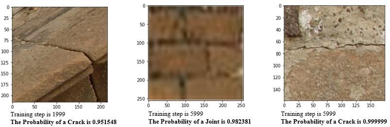
All popular network architectures are composed of above-mentioned basic layers. A
comparison between most used architectures in Table 1 shows performance, depth and
parameter number of those networks: On the one hand, the accuracy for image classification
have been dramatically increased from 1998 to 2015. On the other hand, the architecture of
network become deeper and more complex. In other words, the computer needs to process more
than 60 million parameters to train a model.
 Name LeNet-5 AlexNet VGG GoogLeNet ResNet
 Year 1998 2021 2014 2014 2015
 Top-5-Error - 15.30% 7.30% 6.67% 3.57%
 Data Augmentation - + + + +
 Number of Convolutional Layers 3 5 16 21 151
 Layer Number 7 8 19 22 152
 Parameter Number 6.E+04 6.E+07 1.E+08 7.E+06 6.E+07

 Table 1: Comparing between different CNN architecture (Russakovsky et al., 2015)

After the comparison, LeNet-5 is chosen to be basic architecture in this study for following
reasons: First and most important, it meets the need of computational cost. Second, it has an
acceptable accuracy. LeNet-5 is a classic CNN architecture proposed by Yann LeCun (1998).
It was applied in banking to recognize handwritten numbers on checks. Because of the limited
computing power at that time, grayscale images in 32 ×32 pixel is considered as inputs. LeNet-
5 has 7 layers, 3 of them are convolutional layers. (see Figure 2).

 Figure 2: LeNet-5 architecture (Lecun, Bottou, Bengio and Haffner, 1998)

A number of modifications based on LeNet-5 need to be done to fit this architecture to the
research goal: 1) Instead of one channel (black and white) images of original LeNet-5, the
modified architecture takes three channels colour images as input. All inputs are re-sized into
228×228 pixels to avoid calculation errors, which caused by different image sizes in the dataset.
2) Instead of Sigmoid activation function of original network, which suffers from vanishing
gradient problem, the modified architecture uses ReLU as activation function. 3) Max-Pooling
and Local Response Normalization is used to keep features on the feature map. 4) The single
5x5 CONV layer is replaced by a stack of two 3x3 CONV layer to reduce parameters. A multi-
FC layer set composed of FC1 and FC2 gives the network a stronger expression ability
nonlinear to connect those extracted features from previous layers. 6) During the CNOV
operation, SAME padding technique is used, which uses zeros to pad around the image to make
sure the size of output and input are same. 7) On the end of the network architecture is a
SoftMax layer to calculate the probabilities for each class. The modified network architecture
is shown in Figure 3. Size and Parameters of each layer are shown in Table 2.
 3

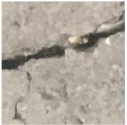
Figure 3: Network architecture for crack-like feature detection

 Input Volume Filter Size Stride Output Volume
 Layer Parameters
 Di Hi Wi K Fx Fy Sx Sy Do Ho Wo
 Input 3 228 228 - - - - - 3 228 228 0
 C1 3 228 228 16 3 3 1 1 16 228 228 448
 P1 16 228 228 3 3 2 2 16 114 114 0
 C2 16 114 114 32 3 3 1 1 32 114 114 4640
 P2 32 114 114 3 3 2 2 32 57 57 0
 FC1 32 57 57 1 - 128 - - 1 128 - 13308032
 FC2 1 128 - 1 - 128 - - 1 2 258

 Table 2: Size and parameters of network architecture for crack-like feature detection

With the parameters trained after the transfer learning process for the target task, the size of
SoftMax layer should also be changed (see Table 3). For example: to make the model able to
different joints and crack in natural stone, the size of SoftMax layer is set to be 3 for different
prediction results, namely cracks, joints and no defects.

 Training goals Size of SoftMax layer
 Detection of the concrete cracks 2
 Detection of natural stone cracks 2
 Differentiation between joints and cracks in natural stone 3

 Table 3: Changes of SoftMax layer for different training goals

Datasets

The concrete cracks dataset (see Figure 4 (a)) contain a total of 40,000 images with 227×227
pixel resolutions (Zhang, 2016). The whole dataset is evenly divided into two groups as positive
crack and negative crack images for classification. Data augmentation like random rotation or
flipping is not used in this dataset. This dataset is divided into a training set with 39600 images
and a test set with 2400 images.

The natural stone cracks dataset (see Figure 4 (b)) contain 150 small images with different
Resolutions. The whole dataset is divided into a test set of 10 images and a train set of 140
images. In the training set, 70 images are labelled with crack and other 70 images are labelled

 4

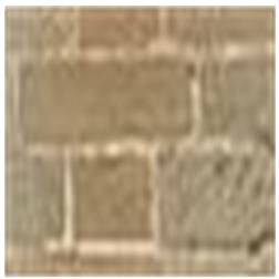
with negative. Different types of cracks are contained in the dataset, such as hair crack and
splitting.

The cracks and joints of natural stones dataset (see Figure 4 (c)) is made of natural stone
contains 150 images with different pixel resolutions. All images related to natural stone cracks
are cut from RGB images with a resolution of 2560×1920. The whole dataset is divided into a
test set of 10 images and a train set of 140 images. The training set consists of 70 pictures with
natural stone crack and 70 pictures with joints. In the test sets, 5 images are natural stone with
cracks and others images are about joints.

 (a) Concrete crack (b) Natural stone crack (c) Joints of nature stones
 Figure 4: Examples of cracks and joints in datasets

Training Process and Results
An overview of training process can be seen from Figure 5: Step 1: Feed the images and labels
into the network. Step 2: Iterate over each example in the training dataset within one step by
grabbing its features and label. Step 3: Compare the prediction of inputs with the real label.
Measure the SoftMax value of the prediction and use that to calculate the model’s loss and
gradients. Step 4: Update the model’s variables with Adam optimizer. Step 5: Repeat for each
epoch. The loss value ls calculated with = . The SoftMax function can be described
with = ⁄ =1
 
 , where is the SoftMax value of element j, is the original value of
the element, and is the number of elements in the vector.

 Figure 5: Training process overview

The Training process of the concrete cracks detection model took 3038 seconds. Figure 6
summarizes the loss and accuracy changes during training process of this model. As can be
seen from Figure 6 (a), those lines in purple and orange show the fluctuation of training loss
and testing loss separately. They both show sharp fluctuation before 10,800 training steps and
trend to become steady after 11,100 training steps. Until 15,000 training steps, the accuracy of
testing gets stable around 100%. Taking the model with 14,199 training steps for example,
when the test loss is near to 0, the test accuracy is near to 1. We hence keep the model with
14,199 training steps for validation and the TF.

 5

Accuracy Training Testing
 Loss Training Testing 100%
0.7 95%
0.6 90%
0.5 85%
0.4 80%
0.3 75%
0.2 70%
0.1 65%
 0 60%

 1500
 2250
 3000
 3750
 4500
 5250
 6000
 6750
 7500
 8250
 9000
 9750
 0
 750

 10500
 11250
 12000
 12750
 13500
 14250
 15000
 1400
 2100
 2800
 3500
 4200
 4900
 5600
 6300
 7000
 7700
 8400
 9100
 9800
 0
 700

 10500
 11200
 11900
 12600
 13300
 14000
 14700
 Training steps Training steps

 (a) Loss (b) Accuracy
 Figure 6: Loss and accuracy changes of concrete crack detection model

 As can be seen in Figure 7(a) for natural stone cracks detection model, the red line stands for
 the accuracy using the TF, and the light purple line stands for the accuracy without using the
 TF. After first 50 training steps, training accuracy of the TF is 87.5%, which is higher than the
 one without (53.12%). Additionally, it took 36 seconds for training with TF to get a training
 accuracy over 97%, while it took 62 seconds for the training without TF. Similarly for Cracks
 and joints detection model, Figure 7(b) shows that TF needs less time (28 seconds) compared
 to normal training (44 seconds) to get an accuracy over 97%.

 (a) Natural stone cracks detection model (b) Cracks and joints detection model
 Figure 7: Comparison between training with and without the TF

 The training process of the natural stone cracks detection model took 367 seconds. Figure 8
 provides data regarding loss and accuracy changes while the model was training. Both training

 6

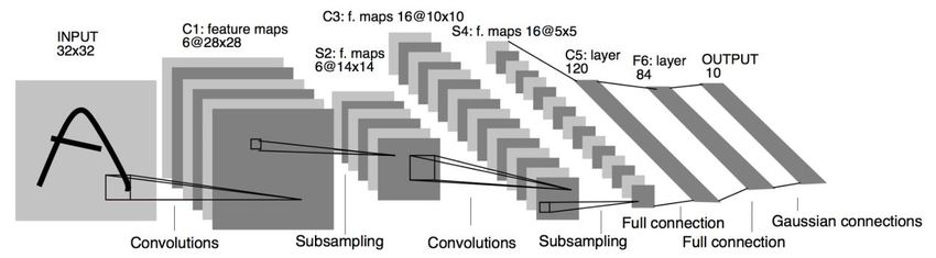
accuracies and testing accuracies keep steady after 150 train steps, where training accuracy is
around 100 % and testing accuracy is around 90 %.

Loss Training Testing Training Testing
 Accuracy
0.7 100%
0.6
 90%
0.5
0.4 80%
0.3 70%
0.2
0.1 60%
 0 50%

 450
 0
 150
 300

 600
 750
 900
 1050
 1200
 1350
 1500
 1650
 1800
 1950
 150
 0

 300
 450
 600
 750
 900
 1050
 1200
 1350
 1500
 1650
 1800
 1950
 Training steps Training steps

 (a) Loss (b) Accuracy
 Figure 8 Loss and accuracy changes of natural stone crack detection model

The training process of the cracks and joints of natural stones detection model took 84
seconds. As can be seen in Figure 9, training accuracy and testing accuracy increase to around
100 % and around 82 separately after 400 steps.

Loss Training Testing Accuracy Training Testing
0.8 100%
 90%
0.6 80%
0.4 70%
 60%
0.2
 50%
 0 40%
 2800
 0
 400
 800
 1200
 1600
 2000
 2400

 3200
 3600
 4000
 4400
 4800
 5200
 5600
 6000

 2400
 0
 400
 800
 1200
 1600
 2000

 2800
 3200
 3600
 4000
 4400
 4800
 5200
 5600
 6000
 Training steps Training steps
 (a) Loss (b) Accuracy
 Figure 9: Loss and accuracy changes of cracks and joints detection model

Results
After loading the concrete cracks detection model with 141999 training steps, Figure 11(a)
and 10 (b) shows the prediction results of a concrete with 0.506732 probability of having no
crack and with 1.000000 probability of having a crack separately. After loading the natural
stone cracks detection model with 1999 training steps, Figure 11(c) and 10 (d) shows the
prediction results of a natural stone with 0.999998 and 0.951548 probability to have a crack
separately.
It should be pointed out that the probability value indicates the confidence degree of the
computer on the prediction result. It is calculated with ⁡ ⁡ = ⁡ − .

 7

(a) Perdition of concrete (b) Perdition of concrete (c) Perdition of natural stone
without crack with crack with crack

(d) Perdition of natural stone (e) Perdition of natural stone (f) Perdition of natural stone
wit crack with joint with crack

 Figure 11: Utilization of the models

 Conclusion and Discussion
The whole study consists mainly of four parts. A lightweight CNN architecture is built. A CNN
model is then trained so that it can detect whether there are concrete cracks in images. After
that, the TF method is used in the training process to train a natural stone detection model with
few training data. Consequently, the training steps and training time to get the comparable result
are significantly reduced. Since there are not only cracks in a natural stone façade, a further
advanced CNN, to promote the usage scenarios of this CNN in renovation works, is trained, so
that the computer is able to distinguish, if there are cracks, joints, or nothing special in the input
image.

From the comparative studies, which also used CNN to detect concrete cracks, this proposed
light weighted CNN architecture shows a possibility to training models on laptops compared to
the Cha (2017). Training time of all three models in this work are within one hour. Also, our
results suggest that the main advantages of transfer learning are the potential of saving training

 8

time as well as solve the problem of insufficient training data (see Figure 7). As shown in results,
our work is demonstrated as an effective tool for the industry use.
Although there are discoveries revealed by this study, there are also limitations. The size of data
set with cracks is quite small, which makes the trained model not robust enough because not all
the features from diverse cracks are including in the dataset. Thanks to the relative lightweight
architecture of our model, we encourage future research to implement our model on mobile
applications, such as smart phone, to make the renovation process more efficient and smoother.

 References
LeCun, Y., Bottou, L., Bengio, Y. and Haffner, P., 1998. Gradient-based learning applied to document
recognition. Proceedings of the IEEE, 86(11), pp.2278-2324.
Krizhevsky, A., Sutskever, I. and Hinton, G.E., 2012. Imagenet classification with deep convolutional
neural networks. Advances in neural information processing systems, 25, pp.1097-1105.
Simonyan, K. and Zisserman, A., 2014. Very deep convolutional networks for large-scale image
recognition. arXiv preprint arXiv:1409.1556.
He, K., Zhang, X., Ren, S. and Sun, J., 2016. Deep residual learning for image recognition.
In Proceedings of the IEEE conference on computer vision and pattern recognition (pp. 770-778).
Szegedy, C., Liu, W., Jia, Y., Sermanet, P., Reed, S., Anguelov, D., Erhan, D., Vanhoucke, V. and
Rabinovich, A., 2015. Going deeper with convolutions. In Proceedings of the IEEE conference on
computer vision and pattern recognition (pp. 1-9).
Cha, Y.J., Choi, W. and Büyüköztürk, O., 2017. Deep learning‐based crack damage detection using
convolutional neural networks. Computer‐Aided Civil and Infrastructure Engineering, 32(5), pp.361-
378.
Kang, D. and Cha, Y., 2018. Autonomous UAVs for Structural Health Monitoring Using Deep Learning
and an Ultrasonic Beacon System with Geo-Tagging. Computer-Aided Civil and Infrastructure
Engineering, 33(10), pp.885-902.
Fukushima, K., 1980. Neocognitron: A self-organizing neural network model for a mechanism of pattern
recognition unaffected by shift in position. Biological Cybernetics, 36(4), pp.193-202.
Glorot, X., Bordes, A. and Bengio, Y., 2011, June. Deep sparse rectifier neural networks. In Proceedings
of the fourteenth international conference on artificial intelligence and statistics (pp. 315-323). JMLR
Workshop and Conference Proceedings.Russakovsky, O., Deng, J., Su, H., Krause, J., Satheesh, S., Ma,
S., Huang, Z., Karpathy, A., Khosla, A., Bernstein, M., Berg, A. and Fei-Fei, L., 2015. ImageNet Large
Scale Visual Recognition Challenge. International Journal of Computer Vision, 115(3), pp.211-252.
Zhang, L., Yang, F., Zhang, Y.D. and Zhu, Y.J., 2016, September. Road crack detection using deep
convolutional neural network. In 2016 IEEE international conference on image processing (ICIP) (pp.
3708-3712). IEEE.
Yosinski, J., Clune, J., Bengio, Y. and Lipson, H., 2014. How transferable are features in deep neural
networks?. arXiv preprint arXiv:1411.1792.
Xiang, Y., Tang, T., Su, T., Brach, C., Liu, L., Mao, S. and Geimer, M., 2020. Fast crdnn: Towards on
site training of mobile construction machines. arXiv preprint arXiv:2006.03169.
Xiang, Y., Wang, H., Su, T., Li, R., Brach, C., Mao, S.S. and Geimer, M., 2020. Kit moma: A mobile
machines dataset. arXiv preprint arXiv:2007.04198.
ASHRAE, (2005). Handbook of Fundamentals. Atlanta: American Society of Heating, Refrigerating
and Air Conditioning Engineers.
Abdel-Qader, I., Abudayyeh, O. and Kelly, M.E., 2003. Analysis of edge-detection techniques for crack
identification in bridges. Journal of Computing in Civil Engineering, 17(4), pp.255-263.
Yeum, C.M. and Dyke, S.J., 2015. Vision‐based automated crack detection for bridge
inspection. Computer‐Aided Civil and Infrastructure Engineering, 30(10), pp.759-770.

 9

Zhou, B., Khosla, A., Lapedriza, A., Oliva, A. and Torralba, A., 2014. Object detectors emerge in deep
scene cnns. arXiv preprint arXiv:1412.6856.
Szegedy, C., Vanhoucke, V., Ioffe, S., Shlens, J. and Wojna, Z., 2016. Rethinking the inception
architecture for computer vision. In Proceedings of the IEEE conference on computer vision and pattern
recognition (pp. 2818-2826).
Smith, L.N., 2017, March. Cyclical learning rates for training neural networks. In 2017 IEEE winter
conference on applications of computer vision (WACV) (pp. 464-472). IEEE.
Khan, S., Rahmani, H., Shah, S.A.A. and Bennamoun, M., 2018. A guide to convolutional neural
networks for computer vision. Synthesis Lectures on Computer Vision, 8(1), pp.1-207.
Kang, D. and Cha, Y.J., 2018. Autonomous UAVs for structural health monitoring using deep learning
and an ultrasonic beacon system with geo‐tagging. Computer‐Aided Civil and Infrastructure
Engineering, 33(10), pp.885-902.
Neto, N. and De Brito, J., 2011. Inspection and defect diagnosis system for natural stone
cladding. Journal of Materials in Civil Engineering, 23(10), pp.1433-1443.
Cs.toronto.edu. 2021. CSC321 Winter 2018.
Satyen, R., 2019. [online] Available at: 
[Accessed 17 May 2020].
Katex NDT Equipment. 2021. UV Magnetic Yoke Flaw Detector - AJE-220 | Katex Ltd. [online]
Available at: 
[Accessed 19 May 2021].
eBay. 2021. Olympus Panametrics Omniscan MX 32 : 128 Ultraschall Phased Feld Pa Flaw | eBay.
[online] Available at: [Accessed 19 May 2021].

 10