Research on Duct Flow Field Optimisation of a Robot Vacuum Cleaner
←
→
Page content transcription
If your browser does not render page correctly, please read the page content below
ARTICLE
International Journal of Advanced Robotic Systems

Research on Duct Flow Field Optimisation
of a Robot Vacuum Cleaner
Regular Paper

Xiao-bo Lai1, Hai-shun Wang1,* and Hua-shan Liu2
1 College of Information Technology, Zhejiang Chinese Medical University, China
2 College of Information Science and Technology, Donghua University, China
*Corresponding author e-mail: shopo@zjtcm.net

Received 21 Sep 2011; Accepted 17 Nov 2011

© 2011 Lai et al.; licensee InTech. This is an open access article distributed under the terms of the Creative
Commons Attribution License (http://creativecommons.org/licenses/by/2.0), which permits unrestricted use,
distribution, and reproduction in any medium, provided the original work is properly cited.

Abstract The duct of a robot vacuum cleaner is the length                  Keywords robot vacuum cleaner, duct, flow field
of the flow channel between the inlet of the rolling brush                 optimisation, CFD, pressure loss, modeling
blower and the outlet of the vacuum blower. To cope with
the pressure drop problem of the duct flow field in a
robot vacuum cleaner, a method based on Pressure                           1. Introduction
Implicit with Splitting of Operators (PRISO) algorithm is
introduced and the optimisation design of the duct flow                    It is known that household cleaning is a series of repeated
field is implemented. Firstly, the duct structure in a robot               and tedious manual tasks, carried out by thousands of
vacuum cleaner is taken as a research object, with the                     people every day. Hence, in the age of rapid
computational fluid dynamics (CFD) theories adopted; a                     developments in science and technologies, how to apply
three‐dimensional fluid model of the duct is established                   these high‐tech achievements to reduce the intensity of
by means of the FLUENT solver of the CFD software.                         labour and improve quality of life is an important issue
Secondly, with the k‐ε turbulence model of three‐                          that should be solved by researchers. In recent years,
dimensional incompressible fluid considered and the                        autonomous mobile robots have come under the spotlight
PRISO pressure modification algorithm employed, the                        of many researchers[1, 2, 3, 4]. In the twenty‐first century, the
flow field numerical simulations inside the duct of the                    successful development of the robot vacuum cleaner has
robot vacuum cleaner are carried out. Then, the velocity                   made possible cleaning the floor automatically. However,
vector plots on the arbitrary plane of the duct flow field                 the pressure drop of the duct inside the robot vacuum
are obtained. Finally, an investigation of the dynamic                     cleaner has a significant influence on cleaning efficiency.
characteristics of the duct flow field is done and defects of              Therefore, how to optimise the duct flow field inside the
the original duct flow field are analysed, the optimisation                robot vacuum cleaner has become particularly important.
of the original flow field has then been conducted.
Experimental results show that the duct flow field after                   The duct of the robot vacuum cleaner is the length of the
optimisation can effectively reduce pressure drop, the                     flow channel between the inlet of the rolling brush blower
feasibility as well as the correctness of the theoretical                  and the outlet of the vacuum blower, which also includes
modelling and optimisation approaches are validated.                       the dust container and other intermediaries. It has a

www.intechweb.org                                                                                    Int JXiao-bo
                                                                                                           Adv Robotic Sy, 2011,
                                                                                                                  Lai Hai-shun   Vol. and
                                                                                                                               Wang   8, No. 5, 104-112
                                                                                                                                          Hua-shan  Liu:   104
                                                                                  Research on Duct Flow Field Optimisation of a Robot Vacuum Cleaner
significant impact on the fluid dynamics performance of the results validate the effectiveness and correctness of
the entire duct system. Traditional duct design methods the modelling in the paper.
mainly rely on the results of a comprehensive survey to
test the duct properties. One disadvantage of these 2. Mathematical model of the duct flow field
approaches is that their design cycles are very long.
Moreover, the testing costs of three‐dimensional flow 2.1 Governing equations
field are very high, because the duct shape is usually
complex. Fortunately, the development of computational The mass conservation equation states the rate of increase
fluid dynamics provides a good way to understand the of mass in the fluid element is equated to the net rate of
flow field distribution and the unsteady transformation flow of mass into the element across its faces.
of the duct for the majority of researchers. Ishtiaque et
al.[5] modified the design of the transport duct and This yields
analysed the air‐flow inside the transport duct with the
computational fluid dynamics (CFD) software FLUENT u v w
after creating the transport duct geometry in the 0, (1)
t x y z
geometrical model software GAMBIT. Then the physical
properties of finer and coarser count yarns made from
modified, as well as conventional, transport ducts were or in more compact vector notation
compared to assess the enhancement of properties with
transport duct modification. Gas‐solid two‐phase flow in
a 180 degrees curved duct was simulated with a standard div u 0, (2)
k‐epsilon model, RNG (Renormalisation Group) based k‐ t
epsilon model, Low‐Re k‐epsilon model and an extended
version of the standard k‐epsilon model was adopted. It where ρ is the density, t is the time, u is the velocity
showed that the RNG based k‐epsilon model predicted vector. u, v, w are the components of the velocity vector u
the flow behaviour better than other models[6]. in the x‐, y‐, z‐direction.
Computational fluid dynamics (CFD) simulations are
performed for convective heat and mass transfer between Eq. (2) is the unsteady, three‐dimensional mass
water surface and humid air flowing in a horizontal conservation at a point in a compressible fluid. The first
three‐dimensional rectangular duct[7]. Moujaes and term on the left hand side is the rate of change in time of
Aekula[8]present new results for numerical predictions of the density. The second term describes the net flow of
air flow and pressure distribution in two commonly used mass out of the element across the boundaries.
elbows. A k‐epsilon turbulence model for high Reynolds
number and k‐epsilon Chen model are used for For an incompressible fluid, the density ρ is constant and
comparative purposes. To validate the CFD results, the Eq. (2) becomes
results of two experimental papers using guided vanes
are compared with a simulated vane run under the same div u 0, (3)
condition. The simulations agreed reasonably well with
published experimental results.
or in longhand notation
The present paper focuses on the duct flow field
u v w
optimisation of the robot vacuum cleaner. The flow field 0. (4)
analysis of original duct structure inside the robot x y z
vacuum cleaner is carried out using the computational
fluid dynamics software FLUENT after creating the duct Newton’s second law states that the rate of change of
geometry in the geometrical model software momentum of a fluid particle equals the sum of the forces
Pro/Engineer. The simulations are done using the k‐ε on the particle. Then, the x‐component of the momentum
turbulence model of three‐dimensional incompressible equation is found by setting the rate of change of x‐
fluid. With the velocity vector plots on arbitrary plane of momentum of the fluid particle equal to the total force in
the duct flow field obtained, the defects of the original the x‐direction on the element due to surface stresses plus
duct structure flow field are analysed. After that, the the rate of increase of x‐momentum due to sources.
duct structure is modified and optimised, and the air‐
flow behaviour is simulated. The total flow rates of the This yields
original duct, as well as the optimised duct, are
compared, and comparisons between the experimental Du p xx yx zx
values and the simulation values are also achieved. All
S mx . (5)
Dt x y z
105 Int J Adv Robotic Sy, 2011, Vol. 8, No. 5, 104-112 www.intechweb.orgIt is not too difficult to verify that the y‐component of the Eq. (9) can be rewritten in the discretisation form as
momentum equation is given by follows:
Dv xy p yy zy [( uA)i 1, J ( uA)i , J ] [( vA) I , j 1 ( vA) I , j ] 0, (10)
Smy , (6)
Dt x y z
following the correction values in Eq. (11)
and the z‐component of the momentum equation by
ui ,J ui*,J di ,J pI 1,J pI ,J
Dw xz yz p zz vI , j v*I , j d I , j pI ,J 1 pI ,J
S mz , (7)
Dt x y z , (11)
ui 1,J ui*1,J di 1,J pI ,J pI 1,J
Where
Du
,
Dv
,
Dw
are the rates of increase of x‐, ui 1,J ui*1,J di 1,J pI ,J pI ,J 1
Dt Dt Dt
y‐ and z‐momentum per unit volume of a fluid particle.
The pressure, a normal stress, is denoted by p. Viscous where
stresses are denoted by τ. The suffix notation τij is applied Ai 1, J
to indicate the direction of the viscous stresses. The
di 1, J
ai 1, J
suffices i and j in τij indicate that the stress component .
acts in the j‐direction on a surface normal to the i‐ A
d I , j 1 I , j 1
direction. aI , j 1
The momentum conservation law is usually expressed as Substitute the discretisation Eq. (11) into Eq. (10), we
the partial differencing equations of the Navier‐Stokes obtain
equation in fluid dynamics. Currently, the simulation
approaches of the Navier‐Stokes (N‐S) equations based
on the Reynolds time average are used to solve the
dA
i 1, J
dA I , j 1 dAi , J dA I , j pI , J
dAi 1, J pI 1, J dA i , J pI 1, J dA I , j 1 pI , J 1 dA I , J pI , J 1 , (12)
problem of the incompressible flow in projects. It can be
written as follows:
u* A i, J
u A *
i 1, J
v A*
I, j
v A*
I , j 1
ui ui u j 2 ui uiu j Eq. (12) can be simplified to
si , (8)
t x j xi xi x j x j
aI , J pI , J aI 1, J pI 1, J aI 1, J pI 1, J aI , J 1 pI , J 1 aI , J 1 pI , J 1 bI , J ,
(13)
where ui u j is the turbulent Reynolds stress, si is the
source term. i, j = 1, 2, 3. where
aI 1, J dA i 1, J
When the ρ and si are known, the solutions of the
aI 1, J dA i , J
simultaneous equations combined Eq. (4) and Eq. (8) are
not unique, ui u j is still unknown. At the moment, aI , J 1 dA I , j 1
.
additional turbulence models of these unknowns are aI , J 1 dA I , j
required to make the solutions of the simultaneous
aI , J aI 1, J aI 1, J aI , J 1 aI , J 1
equations closed. Since the software FLUENT provides a
variety of turbulence models, the k‐ε turbulence model is b
I ,J u A *
u * A v* A v* A
i, J i 1, J I, j I , j 1
chosen in this paper.
The PRISO algorithm, which stands for Pressure Implicit
2.2 Pressure correction equations
with Splitting of Operators[9, 10, 11], is a pressure‐velocity
calculation procedure developed originally for non‐
According to the mass conservation equation and
iterative computation of unsteady compressible flows.
momentum conservation equation, the continuity
PRISO involves one predictor step and two corrector
equation can be written as follows:
steps, and may be seen as an extension of SIMPLE, with a
further corrector step to enhance it. The PRISO algorithm
u v solves the pressure correction equation twice so the
0. (9)
x y method requires additional storage for calculating the
www.intechweb.org Xiao-bo Lai Hai-shun Wang and Hua-shan Liu: 106
Research on Duct Flow Field Optimisation of a Robot Vacuum Cleanersource term of the second pressure correction equation. blades. Other areas are also divided into several blocks
Although this method implies a considerable increase in and meshed with the structured grids to improve the
computational effort, it has been found to be efficient and computational efficiency. The latter comprises the outer
fast[12]. Therefore, the PRISO algorithm is adopted to wall of the blowers and areas around them, using the
simulate the fluid dynamical characteristics of the duct fixed coordinate frame in the calculation process. The
flow field in the robot vacuum cleaner. total grid number of the duct model in the robot vacuum
cleaner generated is about 105 million in the paper.
3. Geometric models and boundary conditions
3.2. Boundary conditions
3.1 Geometric models
The physical parameters of the fluid regions and the solid
The grid models of the duct structure in the robot vacuum regions (such as fluid density, etc.) are constants and the
cleaner are shown in Fig.1, mainly including the inlet, the fluid flow in the duct is steady‐state flow, namely, the
outlet, a rolling brush blower, a vacuum blower and a dust pressure, together with the temperature does not change
container. To reduce the grid number and execution time, with time. The fluid flow medium is air and the
we make some simplification without affecting the atmospheric pressure of the experimental environment is
computational accuracy. However, the key components one standard atmospheric pressure, namely, P = 101325Pa,
(such as the rolling brush blower, vacuum blower, wall, temperature T = 295K, air density ρ = 1.25kg/m3, air
etc.) are modelled without making any simplification. The viscosity μ = 1.79×10‐5N s/m2. The duct inlet is defined to
specific places simplified are shown below: the flow inlet so that the data can be obtained from
(1) The duct system has good sealing properties and there experiments the duct outlet is defined to the pressure
is no air leakage except via the inlet and the outlet. outlet. Suppose that the speed of the fluid in the duct inlet
(2) The vacuum blower is viewed as a part of the duct is uniform, in which the direction is perpendicular to the
system and not discussed separately border, and the back pressure of the duct outlet is zero. The
number of the blades on the rolling brush blower is 6, and
First of all, the “stp” format case is imported from the the rotation direction is counter clockwise with the speed
software Pro/Engineer to the GAMBIT for pre‐processing of 700rpm. The number of the blades on the vacuum
and a closed space computational domain is obtained. blower is 5 and the rotation speed is 15000rpm.
Then, the grid model after pre‐processing is imported
into the STAR‐CCM+ to be checked. If there are no Since the air flow in the duct is not very large, the
geometric errors or gaps, the required volume mesh can compressibility of the air has little influence on the flow
be generated directly. The block method is adopted to behaviour of the fluid and the pressure distribution.
meshing and the whole geometric model is divided into Hence, it can be assumed that the air is incompressible
multi‐blocks. Among them, part of the rolling blower and and the density is constant. In this paper, the solution
the vacuum blower are meshed with the unstructured algorithm to the pressure‐velocity coupling is the PRISO
grid to meet the complicated surface structures of the method, the convection‐diffusion problems are analysed
rotating blades. The internal walls of the blowers are with the standard second order upwind differencing
divided into two regions, including the internal regions scheme. Considering the design requirements of the duct
and external regions. The former contain the blades, in the robot vacuum cleaner, the convergence condition to
rotating shaft and surrounded fluid regions. The rotating be determined is that the errors of all the physical
coordinate frame is applied to the calculation process in quantities should be less than 1×10‐5.
these regions and the speed equals the actual speed of the
Figure 1. Grid models
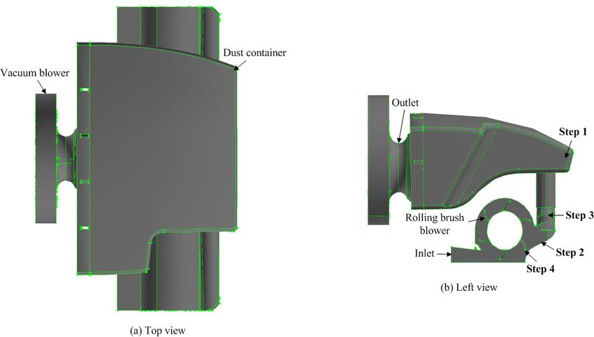
107 Int J Adv Robotic Sy, 2011, Vol. 8, No. 5, 104-112 www.intechweb.orgFigure 2. 3D model of original duct structure
4. Simulation and experimental results analysis
4.1 CFD simulation of the original duct structure
The fluid model shown in Fig.2 is based totally on the
design dimensions of the original duct structure in the
robot vacuum cleaner, which was generated without
making any changes except the simplifications. The
working principle of the robot vacuum cleaner can be seen
from Fig.2. Firstly, the dust particles on the ground are
stirred and raised by the rotating blades of the rolling
brush; then they enter the negative pressure cavity formed
by the blades and the cavity wall of the rolling brush. At
the same time, driven by the rolling brush blades, the dust
Figure 3. Velocity vector plot of the original duct structure
particles can conveniently rush into the junction between
the rolling brush cavity and the dust container. Secondly,
the vacuum blower with high‐speed rotation forms a high
negative pressure chamber in the dust container. Finally,
the dust particles with high‐speed enter the dust container
and gather under the action of the filters. This prevents the
dust particles going into the interior of the vacuum blower
from the inlet and avoids damage to the vacuum blower.
Fig.3 shows the overall velocity vector plot on an arbitrary
plane of the original duct structure in the robot vacuum
cleaner, which is obtained by CFD simulation. It can be
seen from the figure that there is an obvious, large eddy in
the top right of the air intake of the dust container. The
eddy is generated due to the ambiguity of the flow trend
after the air comes into the dust container. At the same Figure 4. Rolling brush blower velocity vector plot of the original
time, the air speed is specially high in the air intake of the duct structure
dust container, resulting in part of the air separating in the
sequent part The eddy formed in this position not only In Fig.4, the sealing property between the top of the
results in higher local flow loss, but would also produce a rolling brush blades and the rolling brush cavity is not
relatively large noise. In this way it reduces the cleaning ideal, resulting in some air along the rotation direction of
efficiency of the duct in the robot vacuum cleaner. the rolling brush blades leaking into the rolling brush
www.intechweb.org Xiao-bo Lai Hai-shun Wang and Hua-shan Liu: 108
Research on Duct Flow Field Optimisation of a Robot Vacuum Cleanercavity from the left of the air intake of the dust container brush blades, which plays a similar role as the jaw.
instead of entering the dust container directly from the air Accordingly, the dust particles are stroked down and
intake of the duct container. This leads to a situation in then enter the dust container from the air intake.
which the air circulation is not ideal and does not easily Step 3: To maximally eliminate the large eddy inside the
form the tip vortex flow and the backflow. Therefore, the duct, the air intake along the axial direction ought to be
original structure should be optimised and improved. made in an eight‐shape trumpet for smooth transition.
Step 4: The rolling brush blades are made into a bent
4.2 CFD simulation of the optimised duct structure shape so that they have the real blower effect
Through the above analysis, the large eddy, tip flow, As is shown in Fig.6, the fluid model of the optimised
backflow and other defects exist in the flow field of the duct structure is simulated through CFD software, the
original duct structure inside the robot vacuum cleaner, boundary conditions remain the same; the overall
which have a great influence on cleaning efficiency. In the velocity vector plot on arbitrary plane of the duct
view of the computational fluid dynamics, the fluid structure can be obtained. We can see from Fig.6 that the
pressure drop is largely caused by the eddy. Therefore, a large eddy in the top right of the dust container has
large‐scale, or even a small, eddy should be avoided been significantly reduced and effectively controlled
when we design the duct structure of the robot vacuum after the duct structure is optimised. Meanwhile, the
cleaner. This means that the duct structure inside the smoothness of the rolling brush cavity transition to the
robot vacuum cleaner should be optimised according to air intake has been improved greatly and the field flow of
the theories of the computational fluid dynamics, the duct structure in the robot vacuum cleaner has been
maximally reducing the energy loss caused by the eddy. perfected.
As is shown in Fig.5, the optimisation scheme of the
original duct structure in the paper is as follows: Fig.7 shows that the sealing property between the top of
Step 1: Minimize the space at the top right of the air the rolling brush blades and the rolling brush cavity wall
intake in the dust container and add a spoiler at the air is better than in the original duct structure, almost no air
intake of the dust container so that the air can enter the along the rotation direction of the rolling brush blades is
dust container just inside the left, avoiding large eddy leaking into the rolling brush cavity from the left of the
production and the pressure drop. air intake in the dust container. The smoothness of the air
Step 2: The internal wall of the air intake in the dust flow is good, which effectively controls the production of
container should be tangent to the top of the rolling the tip flow and the backflow.
Figure 5. 3D model of the optimised duct structure
109 Int J Adv Robotic Sy, 2011, Vol. 8, No. 5, 104-112 www.intechweb.orgFigure 6. Velocity vector plot of the optimised duct structure
Figure 7. Rolling brush blower velocity vector plot of the optimised duct structure
4.3 Validation of calculation results same speed, which verifies the correctness of the duct
structure optimisation in this paper.
Both the original duct structure and the optimised duct
structure are made into physical models and then the Fig.11 (a) shows the comparison between the
total air flow rate from the outlet of the vacuum blower is experimental results and the CFD simulation results of
measured with the air flow meter. The physical model of the total air flux rate from the vacuum blower outlet of
the optimised rolling brush blades, the dust container the original duct structure. Likewise, Fig.11 (b) shows
and the air intake of the dust container are shown in the comparison between the experimental results and
Fig.8, Fig.9 and Fig.10, respectively. Table 1 shows the the CFD simulation results of the total air flux rate from
total air flow rate from the outlet of the original physical the vacuum blower outlet of the optimised duct
model and the optimised physical model under structure. All the results in Fig.11 (a) and Fig.11 (b) are
different speed conditions, respectively. The rotation tested with different rotation speeds of the vacuum
speed of the rolling brush blower maintains 700rpm. It blower. The data comparisons of Fig.11 (a) and Fig.11 (b)
can be seen from Table 1 that the total air flow rate of verify the correctness and the feasibility of theoretical
the optimised physical model is larger than that of the modelling presented in the paper.
original physical model of the duct structure with the
www.intechweb.org Xiao-bo Lai Hai-shun Wang and Hua-shan Liu: 110
Research on Duct Flow Field Optimisation of a Robot Vacuum CleanerFigure 8. Physical model of the optimised rolling brush
Figure 9. Physical model of the optimised dust container
Figure 10. Physical model of the optimised air intake
Rotate speed 10000/rpm 12000/rpm 14000/rpm 16000/rpm
Original structure 49.3/(m3.h‐1) 54.1/(m3.h‐1) 60.9/(m3.h‐1) 66/(m3.h‐1)
Optimised structure 52/(m3.h‐1) 56.5/(m3.h‐1) 61/(m3.h‐1) 69.3/(m3.h‐1)
Table 1. Comparison of total air flow rate from the vacuum blower outlet at different speeds
Figure 11. Total air flow rate comparison between experimental values and simulation values
111 Int J Adv Robotic Sy, 2011, Vol. 8, No. 5, 104-112 www.intechweb.org5. Conclusions [4] Matveev A. S., Teimoori H., Savkin A. V..Navigation
of a unicycle‐like mobile robot for environmental
Aiming at the pressure loss problem of the duct flow field extremum seeking. Automatica, 2011, 47(1): 85‐91.
in the robot vacuum cleaner, by means of computational [doi: 10.1016/j.automatica.2010.10.003]
fluid dynamics and aerodynamics, with the mass [5] Ishtiaque S. M., Singh S. N., Das A., et
conservation equation and momentum conservation al.Optimisation of fluid flow phenomena inside the
equation considered, the duct structure inside the robot transport duct of a DREF‐� friction spinning
vacuum cleaner is taken as a research object in this paper. machine. Journal of the Textile Institute, 2010, 101(10):
The convection‐diffusion problems are analysed with the 906‐916. [doi: 10.1080/00405000903028240]
standard second order upwind differencing scheme and [6] EI‐Behery S. M., Hamed M. H., EI‐Kadi M. A., et
the k‐ε turbulence model of 3D incompressible fluid and al.CFD prediction of air‐solid flow in 180 degrees
the PRISO algorithm are used to carry out the flow field curved duct. Powder Technology, 2009, 191(1‐2): 130‐
numerical simulations of the duct structure in the robot 142. [doi: 10.1016/j.powtec.2008.09.018]
vacuum cleaner. To obtain good dynamic performance, [7] Talukdar P., Iskra C. R., Simonson C. J..Combined
optimisation design based on the analysed results is heat and mass transfer for laminar flow of moist air
achieved. The experimental and simulation results show in a 3D rectangular duct: CFD simulation and
that the method of optimising the duct structure inside validation with experimental data. International
the robot vacuum cleaner can effectively reduce the Journal of Heat and Mass Transfer, 2008, 51(11‐12):
impact on the duct flow field introduced by the large 3091‐3102.
eddy, tip eddy and backflow. The pressure drop is [doi: 10.1016/j.ijheatmasstransfer.2007.08.034]
decreased and the cleaning efficiency of the robot vacuum [8] Moujaes S. F., Aekula S..CFD predictions and
cleaner is improved. What is more, the correctness and experimental comparisons of pressure drop effects of
the feasibility of theoretical modelling presented in the turning vanes in 90 degrees duct Elbows. Journal of
paper are verified, which can overcome the Energy Engineering‐ASCE, 2009, 135(4): 119‐126.
shortcomings of the duct traditional design method. The [doi: 10.1061/(ASCE)0733‐9402(2009)135:4(119)]
conclusions obtained from this paper provide a useful [9] Issa R. I..Solution of the implicitly discretised fluid
reference and practical significance to the research on flow equations by operator‐splitting. Journal of
the aerodynamics characteristics of the duct flow field in Computational Physics, 1986, 62(1): 40‐65.
other robots. [doi: 10.1016/0021‐9991(86)90099‐9]
[10] Park TS. Effects of time‐integration method in a
6. References large‐eddy simulation using the PISO algorithm: Part
I ‐ Flow field. Numerical Heat Transfer Part A‐
[1] Hong J., Park K..A new mobile robot navigation Applications, 2006,50(3): 229‐245.
using a turning point searching algorithm with the [doi: 10.1080/10407780600602374]
consideration of obstacle avoidance. International [11] Kang KG, Ryou HS. Computation of solidification
Journal of Advanced Manufacturing Technology, 2011, and melting using the PISO algorithm. Numerical
52(5‐8): 763‐775. [doi: 10.1007/s00170‐010‐2749‐5] Heat Transfer Part B‐Applications, 2004, 46(2): 179‐194.
[2] Klancar G., Matko D., Blazic S..A control strategy for [doi:10.1080/10407790490438563]
platoons of differential drive wheeled mobile robot. [12] Issa R. I., Gosman A. D., Watkins A. P..The
Robotics and Autonomous Systems, 2011, 59(2): 57‐64. computation of compressible and incompressible
[doi: 10.1016/j.robot.2010.12.002] recirculating flows. Journal of Computational Physics,
[3] Samsudin K., Ahmad F. A., Mashohor S..A highly 1986, 62(1): 66‐82. [doi: 10.1016/0021‐9991(86)90100‐2]
interpretable fuzzy rule base using ordinal structure
for obstacle avoidance of mobile robot. Applied Soft
Computing, 2011, 47(1): 85‐91.
[doi: 10.1016/j.asoc.2010.05.002]
www.intechweb.org Xiao-bo Lai Hai-shun Wang and Hua-shan Liu: 112
Research on Duct Flow Field Optimisation of a Robot Vacuum CleanerYou can also read