Estimating multilevel models for categorical data via generalized least squares
←
→
Page content transcription
If your browser does not render page correctly, please read the page content below
Revista Colombiana de Estadı́stica
                                                Volumen 28 No 1. pp. 63 a 76. Junio 2005

Estimating multilevel models for categorical data
                   via generalized least squares
                           Minerva Montero Dı́az*
                            Valia Guerra Ones**

                                        Resumen
      Montero, Castell & Ojeda (2002) propusieron una estrategia para formular
      modelos multinivel para tablas de contingencia basada en la aplicación del
      modelo lineal general a datos categóricos jerárquicos. Aplicando el método
      a un modelo de regresión logı́stica multinivel con datos simulados, encon-
      tramos que las estimaciones de los parámetros aleatorios son inadmisibles
      en ciertas situaciones, con sesgos grandes y estimaciones negativas de la va-
      rianza cuando los conjuntos de datos son desbalanceados. Para corregir los
      estimadores proponemos una técnica basada en descomposición de valores
      singulares truncados en la solución de mı́nimos cuadrados generalizados para
      estimar los parámetros aleatorios. Mediante simulación mostramos la efecti-
      vidad de la técnica en cuanto a la reducción del sesgo de los estimadores.

      Palabras claves: Modelos multinivel, mı́nimos cuadrados generalizados, va-
      lores singulares truncados.

                                       Abstract
      Montero et al. (2002) proposed a strategy to formulate multilevel models
      related to a contingency table sample. This methodology is based on the
      application of the general linear model to hierarchical categorical data. In
      this paper we applied the method to a multilevel logistic regression model
      using simulated data. We find that the estimates of the random parameters
      are inadmissible in some circumstances; large bias and negative estimates
      of the variance are expected for unbalanced data sets. In order to correct
      the estimates we propose to use a numerical technique based on the Trun-
      cated Singular Value Decomposition (TSVD) in the solution of the problem
      of generalized least squares associated to the estimation of the random pa-
      rameters. Finally a simulation study is presented to shows the effectiveness
      of this technique for reducing the bias of the estimates.

      Keywords: Multilevel models, Generalized least squares, Truncated Singular
      Value.
   * Instituto de Cibernética, Matemática y Fı́sica. Ciudad Habana. Cuba. E-mail: miner-

va@icmf.inf.cu
  ** Instituto de Cibernética, Matemática y Fı́sica. Ciudad Habana. Cuba

                                           63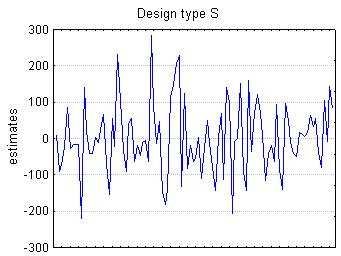
64                                                 Minerva Montero Dı́az & Valia Guerra Ones

1.      Introduction
    The analysis of a sample of contingency tables plays an important role in many
fields of science. Non-normal generalized linear models with random effects have
become increasingly accepted for the analysis of such data (Lee & Nelder (1996,
2001), Breslow & Clayton (1993)). In making inferences from this class of models,
a marginal-likelihood analysis is often troubled by intractable integration. To
avoid this, during recent years, various approximate methods of inference to fit
multilevel models for binary or count data have been proposed (Longford 1994,
Goldstein 1991).
    Montero et al. (2002) consider the GSK approach (Grizzle, Starmerc & Koch
1969), as a tool to formulate multilevel models for analyses a sample of contingency
tables and introduce an estimation procedure that may be applied to fit these
models. This procedure relegates the analysis of a sample of contingency tables
to a class of problem that can be handled by Generalized Least Squares (GLS).
One of the main advantages of the procedure is the similarity with the case of the
multilevel linear model; hence it can be used in situations where other methods
impose the solution of complicated mathematical expressions.
    In this paper the validity of this procedure for the analysis of a sample of
contingency tables is explored by means of a multilevel logistic regression model
with random slope. When the data are balanced (Montero, Castell & Ojeda 2003)
the procedure can obtain estimates of the random parameters at accepted levels of
bias and precision; however, the estimations can be inadmissible when the data are
unbalanced. In this paper, we analyze the theoretical and numerical reasons that
justify the disturbing estimations for the random parameters. The analysis is based
on the effect of the smallest singular values of the design matrix on the random
parameter estimation. We propose the Truncated Singular Value Decomposition
(TSVD) as a technique for avoiding the inadmissible solutions and the L-curve
criterion is suggested for calculating the truncation index. Simulations varying
the degree of imbalance and the variance size of the random effects are presented
to illustrate the effectiveness of the proposed technique.

2.      The Model and Estimation Procedure
     We consider a 2-level hierarchical data structure. Suppose a sample of J
contingency tables (level-2 units) where the rows of each table, called subpop-
ulations, represent I levels (level-1 units) of an explanatory variable or combi-
nations of levels of several explanatory variables. Random samples of size nij
(i = 1, 2, . . . , I; j = 1, 2, . . . , J) are selected from rows. The responses are clas-
sified according to r categories with nilj , (l = 1, 2, . . . , r) denoting the number of
elements classified in the lth response category for the ith subpopulation of the
jth table.
                                                                                p     P
     Let πj = π1j    p
                       , π2j
                          p
                             , . . . , πij
                                        p
                                            , πij = (πi1j , πi2j , . . . , πirj ) with   πilj = 1, repre-
                                                                                   i
sents a vector of probabilities for the jth table. Each set of probabilities has r − 1
Estimating multilevel models for categorical data via generalized least squares          65

linearly independent elements.
                                                         p
    Let F (πj ) = [F1 (πj ) , F2 (πj ) , . . . , F (πj )] be a vector of a < I (r − 1) func-
tions of πj .
    Different types of functions may be represented in a relatively simple manner
using matrix notation ()(Forthoper and Koch, 1973). The function of the probabil-
ities can be simple (e.g., the same probability) or complex (e.g., a rank correlation
coefficient between two response variables, etc).
    By analyzing tables where the I samples of the J tables are independent, the
GSK approach establish that once the function has been specified it can be used
as dependent variable in a linear model. However, when analyzing a sample of
contingency tables, the lack of independence between subpopulations results in
distortion of variance estimates and this can result in problems with type I error
for ordinary test statistic.
    The procedure presented in this paper explicitly takes into account dependence
across tables as well as within tables. The values of the functions of the proba-
bilities become realizations of the dependent variable in a multilevel linear model.
Dependencies between the observations are modeled via random effects. Once the
model is formulated, it is possible to apply the asymptotic theory of estimation in
the framework of the general linear model. The estimation procedure is based on
iterative generalized least squares.

2.1.    Multilevel Model for Proportions
    In this paper we are mainly concerned with the logit function. We consider a
sample of contingency tables with a set of two proportions, pij , 1−pij as outcomes,
for the individuals classified in the ith row from the jth table. The following 2-level
logit model with a single dichotomy explanatory variable is considered:

       fij = logit (pij ) = log (pij ) − log (1 − pij ) = γ00 + γ10 xij + uj zij + eij   (1)

where xij is a covariate having fixed effect γ10 , zij is a covariate having random ef-
fects uij at the 2-level and eij are independent level-1 random errors. The situation
studied in this paper correspond to the case where zij = xij
    We assumed that the observed proportions follow a binomial distribution, but
a simplification was introduced. As suggested by Goldstein (1987) we can simply
required the variances to be inversely proportional to nij , then, the level-1 variance
of fij is also inversely proportional to nij . If we further assume a simple random
variation of the fij across tables, then the between tables variation is assumed to
be the same for each of the I subpopulations.
    We assume that:
                                  E (uij ) = E (eij ) = 0

                                                  σe2i
               V ar (uj ) = σu2 , V ar (eij ) =        and Cov (uj, eij ) = 0
                                                  nij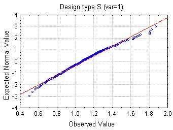
66                                           Minerva Montero Dı́az & Valia Guerra Ones

     An expression for the total variance of fij in the model (1) can be written as:

                                                   σe2i
                                       σu2 zij +
                                                   nij
for the ith subpopulation. The model requires then the estimation of three random
parameters, σu2 , σe20 and σe21 .
    Let pj be the vector of observed proportions, given in the same way as πj .
Note that model (1) can be written as a special case of the general linear mixed
model:
                                  F (p) = XΓ + Zu + e                          (2)
where F (p) = A log (p) is the logit function for the observed proportions, whit
A denoting the matrix of the coefficients of the natural logarithms of the vector
p = (p1 , p2 , . . . , pJ ); Γ is a vector of fixed coefficients with design matrix X; u is a
vector of random effects whit design matrix Z and e is a vector of random errors.
   It should been now be noted that:

     E (F (p)) = XΓ,     Let V ar (e) = Ωe , V ar (u) = Ωu        and     Cov (e, u) = 0

     We can then say that:

                           V ar (F (p)) = VF = ZΩu Z p + Ωe

     The model (2) is a special case of the general linear model:

                                     F (p) = XΓ + e∗

where e∗ = Zu + e, E (e∗ ) = 0 and Cov(e∗ , e∗ ) = VF .
   If the covariance matrix is known, the parameter vector Γ, is estimated by
generalized least squares:

                           Γ = X p VF−1 X X p VF−1 F (p)                   (3)

    When VF is unknown a common practice is to substitute VbF for an estimate
VF in the expression (3). We carry out an iterative procedure analogous to the
described in Goldstein (1995) which alternates between estimates of fixed and
random parameters until convergence. We estimated the fixed parameters from a
generalized least squares (GLS) fit for categorical data ignoring the random errors
at level 2 (see appendix A).
    Once suitable starting values for the fixed parameters are obtained we form the
“raw” residuals Fe = F (p)− ΓA
                             b which can be used to estimate the random parame-

ters in the model. Then form the cross-product matrix E (F ∗ ) = E FeFe = VF .
We vectorize the cross-product matrix F ∗∗ = vec (F ∗ ), and similarly we construct
the vector vec(VF ). The relationship between these vectors can be expressed as
the following linear model involving the random parameter vector θ, so that:

                                     F ∗∗ = Z ∗ θ + R                                    (4)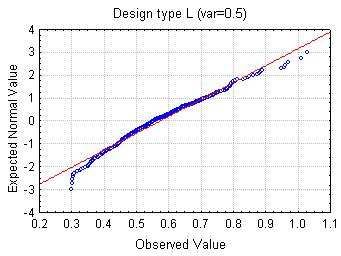
Estimating multilevel models for categorical data via generalized least squares 67
where Ωu and Ωe are the elements of θ, Z ∗ is the design matrix for the random
parameters and R is a residual vector. In order to estimate the random parameter
vector θ, we carry out a generalized least squares analysis, so that:
p −1 −1 p −1
θb = Z ∗ V ∗ Z ∗ Z ∗ V ∗ F ∗∗
where V ∗ is the Kronecker square product of VF , namely V ∗ = VF ⊗ VF . The
estimated covariance matrix for the fixed parameters is:
Cov Γ b = X p V −1 X −1
and for the random parameters:
p −1 −1 t −1 t
t −1 −1
Cov θb = Z ∗ V ∗ Z ∗
−1
Z ∗ V ∗ Cov (F ∗∗ ) V ∗ Z ∗ Z ∗ V ∗ Z ∗
Assuming multivariate normality, Goldstein & Rasbash (1992) show that:
p
p −1
Cov θb = 2 Z ∗ V ∗−1 Z ∗
We observed that in some circumstances the estimation procedure can produce
inadmissible estimates of the random parameters. We consider the case where the
quality of estimations is affected by imbalance among the subpopulation sample
sizes.
3. Analysis of Simulated Data
Simulation studies (Montero et al. 2003) based on the model (1), used to inves-
tigate how the effects of sample size may affect the estimation of the parameters,
show that, the proposed estimation procedure seems to perform adequately for
balanced data, in the situations taken into account.
To explore the properties of estimators for unbalanced data we use the same
hierarchical structure as in the balanced case; i.e., the values of parameters γ00
and γ10 in the model (1) were set to 0.5 and 1.0, respectively. The level-2 random
effects uj are generated from independent normal distribution with zero mean and
finite variance. Logit(πij ) is obtained adding the fixed part and level-2 random
effects. Finally, the values of the variable nij (used for obtain pij ) are generated
from a binomial distribution with parameter πij .
The number of contingency tables is fixed at 50. Several different uniforms
distributions were used to generate the sample sizes of each row in a set of tables.
The designs are classified in four different types of designs depending on the degree
of imbalance of the tables, that is:
Type B: Design Balance, nij = 200 for all i, j.
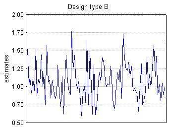
Type S: Design Slightly unbalanced, nij ∼ U (199, 200).
Type M: Design Moderately unbalanced, nij ∼ U (150, 200).
Type L: Design Largely unbalanced, nij ∼ U (100, 200).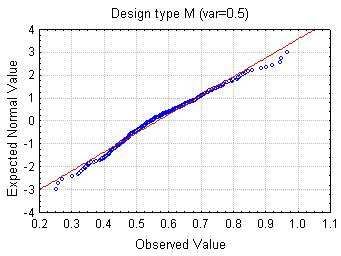
68                                        Minerva Montero Dı́az & Valia Guerra Ones


    One small and one large level-2 variance σu2 = 0.5 and σu2 = 1.0 were as-
sumed. Thus, there are 4×2 = 8 different design conditions and for each condition
100 simulated data sets were generated.
    The estimations of the fixed and random parameters were obtained for sim-
ulations under the different conditions of the designs. The procedure produced
reasonably unbiased estimates for the fixed parameters γ00 and γ10 , but it ex-
hibits big difficulties in the estimates of the random parameters for unbalanced
samples. We focus our attention on the estimates of the variance of the random
                  bu2 . Because of similar behaviors of the estimates, in this section
effects, that is, σ
we only show the case where the random parameter is sufficiently large to be
interesting σu2 = 1 .
    Figure 1 shows plots of the distributions of 100 estimates of the random para-
meters for each design considered in the study. Note that large bias and negative
estimates of the variance are expected for the three unbalanced data sets. The
situation is particularly bad when the tables are slightly unbalanced. In contrast,
the estimates for tables more unbalanced appear to be less biased, but are still
inadmissible. Paradoxically, the biggest differences are between the balanced set
data and the slightly balanced.

Figure 1: Line plot of the distributions of 100 estimates of the random parameters
for the four designs considered.
Estimating multilevel models for categorical data via generalized least squares    69

4.     Understanding and Solving the
       Numerical Difficulties
    The origin of the inadmissible estimates of the random parameters for unbal-
anced data is related to the numerical solution of the general linear model (4).
    Consider the Cholesky decomposition of the symmetric positive definite covari-
ance matrix τ 2 V ∗ = BB t . Then, the solution vector θ in (4) can be calculated
solving the least square problem:
                              min B −1 (Z ∗ θ − F ∗∗ )         2
                                                                                  (5)

    This problem should be solved using a stable algorithm suggested by Paige
(1979), where the pseudoinverse of B is not calculated implicitly. However, if B is
a well-conditioned matrix an obvious computational approach
                                                                to this problem is
to apply any standard technique to minimize B −1 Z ∗ θ − B −1 F ∗∗ .
    The Singular Value Decomposition (SVD) is a useful tool to solve (5) and
to understand the numerical results shown in Figure 1. Given the matrix W =
B −1 Z ∗ , it always exists orthonormal matrices U and V and a diagonal matrix S
such that:
                                     W = U SV p
the diagonal elements Si of S are called singular values of W .
   Using the SVD of W , the random parameter vector θ in (4) can be written as:
                                      rank(W )
                                        X        Uip F ∗∗
                                 θ=                       Vi                      (6)
                                        i=1
                                                   Si

where Ui and Vi are the columns of the matrices U and V , respectively, and
rank(W ) denotes the rank of W .
    Expression (6) permits to understand the numerical results shown in Figure 1.
Note that if the matrix W has very small singular values Si ; then the corresponding
coefficients (Ui F ∗∗ | Si ) can increase drastically the magnitude of the solution θ.
Likewise, the presence of small singular values in the matrix W can produce huge
changes when the coefficients of W are slightly perturbed.
    In the simulation study of section 3, we have observed that in the case of
balanced data, the singular values of matrix W are not small, except one of them,
that is smaller than the computer precision. It means the matrix is rank one
deficient and the summand corresponding to the smallest singular value is not
considered in (6). It explains the acceptable estimates obtained for the random
parameters when the data are balanced. However, in the unbalanced cases, where
large bias and negative estimates of the variance are obtained, we observe the
presence of very small singular values Si in the matrix W that are not considered
as zero by the computer and then the summands corresponding to these singular
values are included for calculating θ in the expression (6).
    A possible way to obtain acceptable values for the random parameter vector
θ is truncating the expression (6) to include only the k summands corresponding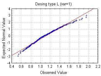
70                                           Minerva Montero Dı́az & Valia Guerra Ones

to singular values greater than a given tolerance. In other words, the random
parameter vector θ is approximated by:
                                       k
                                       X U p F ∗∗
                                              i
                                  θ=                Vi                             (7)
                                       i=1
                                               Si

    This technique is known as Truncated Singular Value Decomposition (TSVD),
(Golub & Loan 1996).
    The determination of the tolerance parameter can be a difficult task. When
there is a well-determined gap between large and small singular values, the para-
meter k is chosen equal to the number of the large singular values. However, when
all singular values decay gradually to zero, and there is no gap in the singular value
spectrum, the parameter k should be calculated using a numerical technique, for
example the L-curve criterion, (Hansen 1998).
    This criterion is based on the determination of the corner of a discrete para-
metric plot of thenorm of the solution θk versus the norm of the corresponding
residual B −1 Z ∗ θk − B −1 F ∗∗ , see details in Hansen (1998).
    It is important to say that other approximations for θ can be considered for
avoiding the overestimation and underestimation of the random parameters. The
main idea is to filter the contribution of each summand of the expression (5) to
the calculated vector. This aspect will be analyzed in future studies. Next section
illustrates the numerical results obtained using the expression (7) and taking the
tolerance parameter as 10−5 .

5.    Simulation Study
    In order to study the performance of the correction introduced, we now simulate
data under the same conditions as one of the preceding simulation study of section
3 and fit the multilevel model (1) by the modified procedure. For every model
specification, 500 data sets were generated. The estimation procedure converged
in all 3000 simulated data sets.
    To analyze the parameter estimates two criterions, bias and efficiency, are
used. Tables 1 and 2 display for each parameter the true value and the values
of the estimated fixed and random parameters averaged over the 500 simulations
conducted every design. The mean of the correspondent Mean Squared Errors
(MSE), and the mean of estimated standard errors are also given. First we discuss
the case where the variance of random effects is large σu2 = 1.0 .
    As we can see from Table 1, it is evident that the application of the Trun-
cated Singular Value Decomposition improves substantially the random parame-
ter estimates. The procedure gives good estimates for the fixed parameters and
reasonably biased estimates for the random parameters at level 2.
    It is clear that the fixed parameter estimates are close to their true value;
that is, the bias of the estimates is small. For the fixed parameters the approach
performs excellently with a bias of 3.7% at the most. Table 1 shows that the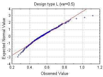
Estimating multilevel models for categorical data via generalized least squares         71

Table 1: Mean values of multilevel logit estimates for 500 simulated data sets for
model (1) assuming σu2 = 1.0
                        Parameters      True value     Estimate     MSE           e.s
    Design type S
                             γ00            0.5          0.505      0.001     0.024
                             γ10             1           1.031      0.025     0.150
                             σu2             1           1.114      0.073     0.124
    Design type M
                             γ00            0.5          0.503      0.000     0.022
                             γ10             1           1.026      0.023     0.148
                             σu2             1           1.082      0.065     0.123
    Design type L
                             γ00            0.5          0.504      0.000     0.020
                             γ10             1           1.014      0.020     0.148
                             σu2             1           1.088      0.065     0.124

estimation procedure results in very small MSE for the fixed parameters, especially
for γ00 .
    The random parameter estimates represent a considerable improvement, but
are still subject to a small bias. The estimates for the three unbalanced data sets
are 11.4, 8.2 and 8.8 percent upward bias respectively. The standard deviation
of estimates is small and none of these biases are statistically different from zero.
The MSE values reported in Table 1 show that the procedure is less efficient in
estimating the random parameters.    Table 2 shows that when the variance of the
random effects is small σu2 = 0.5 none of the estimates is significantly biased.
The estimates of the parameter σu2 are 14.4, 12.8 and 9.4 percent upward biases.

                                                          bu2 .
                       Figure 2: Boxplots of estimates of σ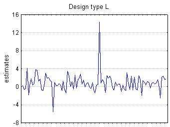
72                                       Minerva Montero Dı́az & Valia Guerra Ones

Table 2: Mean values of multilevel logit estimates for 500 simulated data sets for
model (1) assuming σu2 = 0.5
                       Parameters     True value     Estimate     MSE       e.s
     Design type S
                           γ00            0.5          0.502     0.001    0.024
                           γ10             1           1.022     0.012    0.109
                           σu2            0.5          0.572     0.023    0.083
     Design type M
                           γ00            0.5          0.504     0.000    0.022
                           γ10             1           1.023     0.013    0.108
                           σu2            0.5          0.564     0.019    0.083
     Design type L
                           γ00            0.5          0.502     0.000    0.021
                           γ10             1           1.010     0.012    0.106
                           σu2            0.5          0.547     0.018    0.082

     Finally, we consider how the quality of estimation is affected by the imbalance
of the data when the TSVD is applied. The values of MSE reported in Table 1
and 2 show that the estimator is equally efficient for the three unbalanced designs.
Figure 2 shows graphically the sampling distributions for the estimations of each
design. A general suggestion of this figure is that estimation of random parameters
is little affected by the imbalance of the tables. Quality of estimation seems fairly
insensitive to unbalance.
     Figure 3 shows the normal probability plots of the random parameter estimates
produced by the proposed method. Except for a few outliers the plots for all the
estimates are reasonably consistent with the expected asymptotic normality.

6.    Conclusions
    Our aim was to examine the behavior of an estimation procedure based on
the generalized least squares method for categorical data analysis, in the frame of
multilevel models related to a two-level hierarchical data structure coming from
a sample of contingency tables. We are particularly interested in the multilevel
logistic regression model, but the method can be applied to other models and in
situations where other methods impose the solution of complicated mathematical
expressions. The main advantage of this approach is the similarity with the case
of the linear model.
    On the basis of a number of simulations the results revealed that the degree of
imbalance of the data has an important impact on the estimation of the random
parameters. For unbalanced data, the proposed procedure produces inadmissible
estimates of the random parameters. We showed that the TSVD, used to solve the
Estimating multilevel models for categorical data via generalized least squares 73
bu2 .
Figure 3: Normal Probability Plot of σ74 Minerva Montero Dı́az & Valia Guerra Ones
least squares problem associated to the estimation of the random parameters, can
considerably improve the estimates. The study was carried out via a simulations
study. Random parameters are estimated at accepted levels of bias and precision
after the modification is applied. In summary, TSVD is effective in reducing the
bias of random parameters.
For the specifications considered, the comparison between the designs shows
that the degree of imbalance seems to have neither a systematic nor a significantly
different effect on bias and efficiency of the estimates if a modification, such as the
TSVD, is applied. When variance is small , the estimator was found to be slightly
more efficient that when the variance is large.
Although it is not appropriate to draw general conclusions from a single sim-
ulation study, the results suggest the described procedure should be used as an
efficient method to handle multilevel models for hierarchical categorical data. A
further analysis of more complex models and extreme data sets is necessary to rec-
ommend this approach as a unified approach for modeling a sample of contingency
tables.
Acknowledgements
We would like to thank Dr. Jesús E. Sánchez for his careful reading and
suggestions on the first version of this paper.
A. GLS Fit for Categorical Data
(or GSK Approach)
Consider the data structure of section 1. If we assume the I subpopulations
of the jth table as being uncorrelated with one another a consistent estimator for
the covariance matrix of pj is the matrix:
Vj (pj ) = diag (V1j (p1j ) , V2j (p2j ) , . . . , VIJ (pIj ))
with the matrices:
1
Vij (pij ) = Dpij − pij ppij , (i = 1, 2, . . . , I)
nij
where Dpij is a matrix diagonal with elements of the vector pij on the main
diagonal.
Let Fj ≡ F (pj ). We assume that Fj has continuous second order partial deriv-
atives in an open region containing πj . A consistent estimator for the covariance
matrix of Fj is the matrix:
VbFj = Hj Vj (pj ) Hjp
where H = [∂F (πj ) /∂πj | πj = pj ] is the a × Ic matrix of first partial derivatives
of the functions Fj evaluated on pj .Estimating multilevel models for categorical data via generalized least squares 75
Observations from different tables are mutually independent and, if no function
combines probabilities from more than one population, this independence is main-
tained through the transformation. Thus, the covariance between observations
from different tables is zero, and the estimated covariance matrix of F ≡ F (p) has
the form:
VbF = diag VbF1 , VbF2 , . . . , VbFJ
The GSK approach applies to linear models for F of the form F (π) = XΓ.
Note: A consistent estimator for the covariance matrix of the function F (pj ) =
Bj log (pj ) (Forthofer & Koch 1973) is the matrix:
h i
VbFj = Aj Dj−1 Vcj (pj ) D−1 A−1
j j
where Dj contains the elements of the vector pj on the main diagonal.
References
Breslow, N. E. & Clayton, D. G. (1993), ‘Approximate inference in generalized
linear mixed models’, American Statistical Association 88, 9–25.
Forthofer, R. N. & Koch, G. G. (1973), ‘An analysis for compounded functions of
categorical data’, Biometrics 29, 143–159.
Goldstein, H. (1987), Multilevel Models in Educational and Social Research,
Charles Griffin.
Goldstein, H. (1991), ‘Nonlinear multilevel models, with an application to discrete
response data’, Biometrika 78(1), 45–51.
Goldstein, H. (1995), Multilevel Statistical Models, 2 edn, Halsted Press.
Goldstein, H. & Rasbash, J. (1992), ‘Efficient computational procedures for the
estimation of parameters in multilevel models based on iterative generalized
least squares’, Computational Statistics and Data Analysis 13, 63–71.
Golub, G. & Loan, C. F. V. (1996), Matrix Computations, 3 edn.
Grizzle, J. E., Starmerc, F. & Koch, G. (1969), ‘Analysis of categorical data by
linear models’, Biometrics 25, 489–504.
Hansen, P. C. (1998), Rank-deficient and discrete ill-posed problems: Numerical
aspects and linear inversion, Society for Industrial and Applied Mathematics.
Lee, Y. & Nelder, J. A. (1996), ‘Hierarchical generalized linear models’, Royal
Statistics Society B(58), 619–678.
Lee, Y. & Nelder, J. A. (2001), ‘Hierarchical generalized linear models: a synthesis
of generalized linear model and structured dispersion’, Biometrika 88, 987–
1006.76 Minerva Montero Dı́az & Valia Guerra Ones
Longford, N. (1994), ‘Logistic regression with random coefficients’, Computational
Statistics and Data Analysis 97, 1–15.
Montero, M., Castell, E. & Ojeda, M. M. (2002), Modelos multinivel de una mues-
tra de tablas de contingencia utilizando el enfoque gsk, Technical Report
2002–167, Reporte de investigación del ICIMAF.
Montero, M., Castell, E. & Ojeda, M. M. (2003), Modelos multinivel para una
muestra de tablas de contingencia: un estudio por simulación, Technical Re-
port 2003–228, Reporte de investigación del ICIMAF.
Paige, C. C. (1979), ‘Fast numerically stable computations for generalizad lin-
ear least squares problems’, Society for Industrial and Applied Mathematics
1(1), 165–171.You can also read