Guidance Note on estimating the uncertainty of emission reductions using Monte Carlo simulation - Version 1.0 September 2021

Guidance Note on estimating the uncertainty of
emission reductions using Monte Carlo simulation

 Version 1.0
 September 2021

 1

Contents

Step 1. Identify sources of values used in the emission reduction estimates and whether
they are independent or shared. ................................................................................................ 2

Step 2. Identify the uncertainty associated with each of these variables. ............................ 5

Step 3. Propagate the uncertainties in the estimate of emission reductions using Monte
Carlo simulation .......................................................................................................................... 7

Step 4. Evaluate the contribution of each source to the overall uncertainty ..................... 15

Annex 1. Monte Carlo Example in Excel ................................................................................ 19

Annex 2. Monte Carlo Example in R ....................................................................................... 26

 1

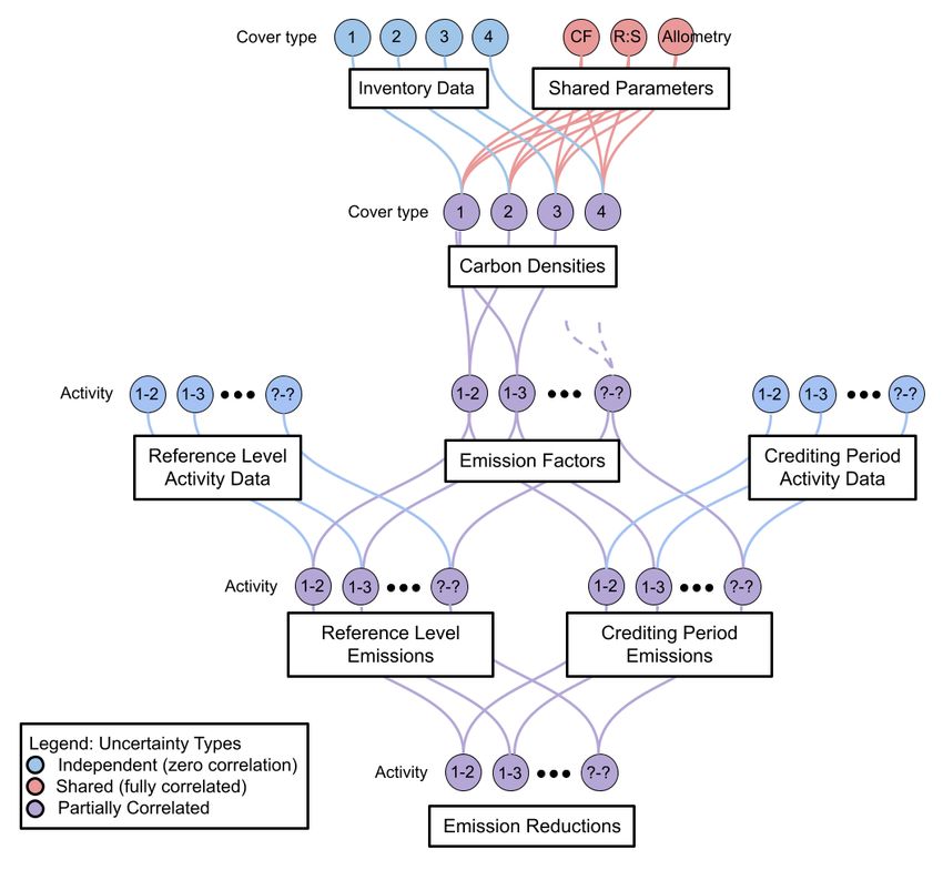
Guidance Note on estimating the uncertainty of emission reductions using
Monte Carlo simulation

 This guidance note has been prepared by the QUERCA (Quantifying Uncertainty Estimates
 and Risk for Carbon Accounting) project at SUNY College of Environmental Science and
 Forestry using funding from the FCPF

Criterion 9 of the FCPF Methodological Framework requires that the uncertainty of the estimate
of Emission Reductions be quantified using Monte Carlo methods. The FCPF Guidelines on
Uncertainty Analysis of Emission Reductions describe which sources of uncertainty to
propagate and provide guidance for conducting Monte Carlo simulations.
ER Programs differ in both the activities they consider and the methods by which they calculate
emission factors and activity data. The sources of uncertainty thus differ, and the calculations
for correctly combining them will also differ. This document describes the general approach and
provides a simple example to illustrate the approach. The general approach described here
includes the following steps:
 ● Step 1. Identify sources of values used in the emission reduction estimates and whether
 they are independent or shared
 ● Step 2. Identify the uncertainty associated with each of these variables
 ● Step 3. Propagate the uncertainties in the estimate of emission reductions using Monte
 Carlo simulation
 ● Step 4. Evaluate the contribution of each source to the overall uncertainty

The simple example has been provided in Excel and in R to help users to understand this
guidance and each of the steps. Each situation is unique, and the examples given will need to
be adapted to the programs in question, but the underlying principles are universal. More details
on the example are provided in Annex 1.
This guidance note complements the FCPF Guidelines on Uncertainty Analysis.

Step 1. Identify sources of values used in the emission reduction
estimates and whether they are independent or shared.
Following the process by which ER Programs estimated emission reductions, programs should
identify all the variables used in the estimation of emissions and removals. Table 1 in the FCPF
Guidelines on Uncertainty Analysis provides a list of the main sources of uncertainty that, at
minimum, shall be evaluated. In the Monte Carlo simulation, the uncertainties in these variables
will be combined by sampling from the likely distributions of their values as determined in Step 2
below.
To combine the uncertainties of multiple variables correctly, requires understanding which
variables are used independently and which are shared across multiple calculations.

Variables and their associated uncertainty sources contribute independently to a particular
calculation if they are independently derived and are not used for any other variable. For
example, tree inventory data are generally collected independently for each stratum or land
cover type and are not used in the calculations for other strata or land cover types (shown in
blue in Figure 1.1).

Other variables and their associated uncertainties are shared across multiple calculations, for
example, carbon fraction (CF), root:shoot ratio (R:S), and tree allometry variables might be used

 2

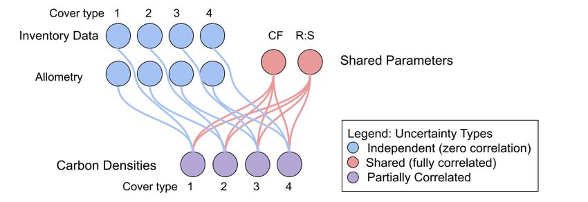
across multiple forest types (shown in red in Figure 1.1). In that case, carbon densities are
calculated by a combination of independent and shared sources and are thus partially
correlated (shown in purple in Figure 1.1) and it is important to represent these correlations
properly when combining them in error propagation.

 Figure 1.1 In calculating carbon densities, inventory data collected in four types of land cover
 are independent (blue). If the same values of carbon fraction (CF), root:shoot ratio (R:S), and
 tree allometry are used across multiple forest types, these are shared (red). Uncertainties
 calculated from a combination of independent and shared sources will be partially correlated
 (purple), with correlation coefficients intermediate between 0 (fully independent) and 1 (fully
 shared).

Whether an uncertainty source should be treated as shared or independent depends on how it
was collected and how it is used in the calculation. Some programs collect tree allometry data
independently for each land cover type. In that case, uncertainties in tree allometry would be
independent for each cover type (Figure 1.2). Theoretically, carbon fraction and root:shoot
ratios could be determined independently for each cover type, or a single value could be used
across forest types. The conversion of carbon to CO2 is treated as a constant without
uncertainty, because variability in carbon and oxygen isotope ratios is negligible.

 Figure 1 2. Whether a variable is independent or shared depends on how the data were
 collected. If allometric equations are specific to each cover type, they are independent. Carbon
 fraction and root:shoot ratio could be determined separately for each forest type, but if they are
 not, they are shared.

Since the emission reductions are estimated as the difference between the reference level of
emissions and the actual monitored emissions, correlation is also relevant between the two
estimates. For example, if programs use the same emission factors in the reference and

 3

monitoring periods, they should be treated as shared (as shown in Figure 1.3). In contrast, if
inventory data are collected independently for each time period, the emission factors for the two
periods are more independent.

 Figure 1 3. Emission factors are derived from carbon densities of the categories of land cover in
 transition. Many such transitions are possible and the number and degree of correlation of such
 activities will differ by program depending on the design. Emission factors may be shared
 between the reference level and monitoring period, as shown here. In estimating the uncertainty
 in the emission reductions, shared sources of uncertainty will share a randomly sampled value
 at each iteration of the Monte Carlo simulation. Uncertainties associated with results based on
 both shared and independent sources will be partially correlated (shown in purple).

The degree of partial correlation (i.e., the value of the correlation coefficient) that arises from
combining a mix of shared and independent uncertainty sources can be estimated analytically
(not covered in this guidance) or by examining the results of Monte Carlo simulation. It is not
important to know the correlation coefficient of intermediate variables in the calculation.
However, if the calculation were to begin with partially correlated inputs, such as carbon
densities, the correlation coefficients would need to be estimated to be propagated correctly
(see Section 3.2.3).

 4

Potential Pitfalls
Treating uncertainty sources as independent when they are shared will underestimate the true
combined uncertainty. In the Simple Example provided in Annex 1, the uncertainty in the ER
should be 416%. If the emission factors are treated as independent between the reference
level and the monitoring period, instead of shared, then a value of 403% is obtained, which is
incorrect.

Step 2. Identify the uncertainty associated with each of these variables.
Using the Monte Carlo approach to error propagation requires defining the distributions of the
variables used in the calculation. There are two ways to generate random samples that mimic
the likely distribution of a variable. The first is to sample from a defined distribution (a probability
density function or PDF). The second is to randomly sample values of the variable from a data
set (bootstrapping).

2.1 Decide between PDF and bootstrap
It is easier to sample from a defined distribution than to sample from a data set, especially in
Excel. Sampling from a data set has the advantage that no assumptions are required about the
nature of the distribution. If the distribution is not normal, then bootstrapping would be more
accurate, unless the data are not representative. The figure below provides a simple decision
tree to decide between PDF and bootstrap to generate random samples that mimic the likely
distribution of a variable.

 Figure 2.1. Decision tree for choosing whether to sample from data or from a PDF.

 5

2.2 Describing uncertainty with a probability density function (PDF)
A mathematical function can be used to describe the distribution of possible values of a
variable. Commonly, in the absence of information to the contrary, normal distributions are
used. A distribution other than normal could be selected if the possible values are not normally
distributed. For some applications, beta, binomial, gamma, weibull, or lognormal distributions
best describe the distribution of observations. However, if there are enough data to determine
that the distribution is not normal, then bootstrapping is also an option.
In REDD+ carbon accounting, uniform distributions have sometimes been used to describe
possible values of the carbon fraction (IPCC 2006 Table 4.3) and root:shoot ratio (IPCC 2019
refinement of 2006 Table 4.4). For this reason, we provide guidance on how to use a uniform
PDF. However, it seems implausible that there is a zero probability of a value outside these
ranges. Instead, we recommend that the mean and standard error of the available data be
used to define a normal distribution. Alternatively, the values could be sampled by
bootstrapping.
In the absence of reliable data, expert judgement may be used to define a PDF. The FCPF
Guidelines on Uncertainty Analysis of Emission Reductions recommends independently
consulting at least three experts when the parameter estimate is not available or is not
representative (e.g. based on research plots). The mean and standard error of the mean of
expert opinions should be used to define a normal distribution. Using the range would be
sensitive to extreme values, and doubling the range (as currently recommended in the
Guidelines) would inflate the uncertainty of the emission reductions. Alternatively, the values
could be sampled by bootstrapping.

2.3 Using the distribution of the data (bootstrapping)

An alternative to representing the distribution of the inputs analytically is to resample the data, a
procedure known as bootstrapping (Ephron and Tibshirani 1994) that is illustrated in figure 2.2.
Values are randomly drawn from the data to create alternative possible data sets with similar
distributions and the same number of observations. Each random sample is drawn from all
possible samples (this is called “sampling with replacement”) because sampling without
replacement, if drawing the number of observations in the data set, would return the original
data set every time. This approach requires no assumption of a distribution and is thus most
true to the measured population. Bootstrapping is especially advantageous when the
distribution is difficult to define. The drawback to this approach is that the representation of the
population is only as good as the data, and if the data set is small, it may not accurately capture
the range of potential values.

 6

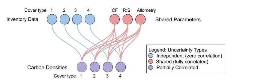
Figure 2.2. Random sampling of values from a data set. The data set has 7 values, which can be
 randomly sampled (with replacement) to create alternative possible data sets.

Potential Pitfalls
Bootstrap sampling must be configured to match the sampling design. For example, if the
sampling design is stratified, it would be necessary to bootstrap for each stratum separately and
produce the overall estimates by combining the stratum information. There could be similar
issues for cluster sampling.
Often data are not representative, due to access to sampling locations (close to roads or forest
edges), or ease of measurement (excavating roots of small trees). This is a potential pitfall both
for characterizing the data with a PDF and for bootstrapping. In these cases, expert judgement
should be used to correct for bias in the data.

Step 3. Propagate the uncertainties in the estimate of emission
reductions using Monte Carlo simulation
The FCPF requires the use of Monte Carlo simulation to quantify the effects of uncertain inputs
on the uncertainty of carbon emission reductions. Using this approach, the calculation of the
emission reductions is iterated hundreds or thousands of times, with the inputs varying
randomly to mimic the uncertainties in the values of all the variables that went into the
calculation of both the Reference Level and the monitored emissions and removals. As
described above in Step 2, random samples that mimic the likely distribution of a variable can
be generated using a defined distribution (a PDF) or by randomly sampling values of the
variable from a data set (bootstrapping). The distribution of the resulting hundreds or thousands
of outputs reflects the net effects of the uncertainties in the inputs.

3.1 How to randomly sample from a distribution or a dataset

 7

3.1.1 Sampling from a distribution
For simulating the uncertainty in an input using a defined distribution, the parameters describing
the distribution are used to generate the random samples.

Distribution Spreadsheet formulas R code

Uniform RAND() generates random numbers uniformly Generate n uniform random
 distributed between 0 and 1. numbers between a1 and a2
 using:
 Generate uniform random numbers between values in
 A1 and A2 using:
 runif(n, min = a1, max = a2)
 = ($A$1 + RAND()*($A$2-$A$1))

Normal NORM.INV(probability, mean, sd) gives an inverse of Given the mean and
 the normal cumulative distribution, at a specified standard deviation (sd) of the
 probability, mean, and standard deviation (sd). distribution, generate n
 random samples using:

 Combining RAND and NORM.INV gives a random
 sample from a distribution with a specified mean and rnorm(n, mean, sd)
 standard deviation. If the mean and sd are in cells B1
 and B2, use:

 =NORM.INV(RAND(), $B$1, $B$2)

 3.1.2 Sampling from a dataset (bootstrapping)
For simulating the uncertainty in an input using bootstrapping, each random sample is selected
from the data set of possible inputs.

 Spreadsheet Formula R code

 If 10 data points are in cells A1:A10, you can Given a sample of size n: (c1,c2,c3,...,cn), you can
 randomly sample 1 of them using: generate a vector:
 =INDEX($A$1:$A$10,ROWS($A$1:$A$10)*R
 AND()+1,COLUMNS($A$1:$A$10)*RAND()+1)
 SampleC

BootstrapSam

For shared sources, the random sample of an For sources (SourceA and SourceB) that are
 uncertainty input is shared: shared, the random sample for the input will be
 shared by both sources for each iteration of the
 Monte Carlo simulation.
 SourceA:
 A3=NORM.INV(RANDARRAY(1, Considering a shared source normally distributed:
 n),$A$1,$A$2) SourceA has mean=mA and sd=sdA
 SourceB:
 B3=$A$3 You can generate n random numbers of SourceA
 as follows:

 In this example, iterations are in rows, and
 SimNumA

Spreadsheet Formula R code

1. For covariance between two vectors X (A1:A30) Load the MASS package, which can develop
and Y (B1:B30), a 2 x 2 variance-covariance matrix multivariate normal random numbers:
will be needed.

 library(MASS)
Matrix A

 First generate a 2 x 2 variance-covariance
 X Y
 matrix between vectors X and Y

 X =VAR.S(A1:A30) =COVARIANCE.S(A1:
 A30,B1:B30) A

4. Calculate a random bivariate normal vector. For n
 random number iterations, this would be a 2 x n
 matrix with the same formula in each cell. Highlight
 cells to form a 2 x n matrix, type the formula:

 =MMULT(C NORM.INV(RANDARRAY(2,n))+B
 After typing the formula, pressing ctrl + shift + enter
 on the keyboard will fill all of the cells in the matrix
 with the function.
 Each cell in the random bivariate normal vector is the
 mean of that variable plus a random residual with the
 desired correlation.

3.3 How to iterate
Random sampling, whether from a PDF or from data, can be repeated many times to generate
a distribution of estimates from which the uncertainty can be assessed.

 Spreadsheet Formula R code

 Each calculation is repeated in rows (or columns). In the case of a normal distribution with a specified
 mean (mean) and standard deviation (sd), a
 random number can be generated as follows:
 Excel 365 has a RANDARRAY function which
 facilitates this process.
 rnorm(1,mean,sd)
 The RANDARRAY formula is used in combination
 with the formula used to sample from the data.
 RANDARRAY(R,C) R uses matrices and arrays to store data.
 Repeated calculations are handled by the number
 where R is the specified number of rows and C is
 of elements in the array (n). To generate n random
 the specified number of columns. For example, if
 numbers, indicate n:
 you are doing iterations in rows, R refers to the
 number of iterations, and C is 1.
 rnorm(n,mean,sd)
 For example, if sampling from a normal distribution
 with mean in cell A1, sd in cell A2, and the number
 of iterations in cell A3,
 = NORM.INV(RANDARRAY($A$3,1),
 $A$1, $A$2)

 The advantage of RANDARRAY is that the formula
 is represented only once, instead of separately in
 each iteration. Having thousands of formulas
 makes the file enormous and the execution slow.
 You should probably invest in Office 365 if you
 want to do Monte Carlo in Excel.

 12

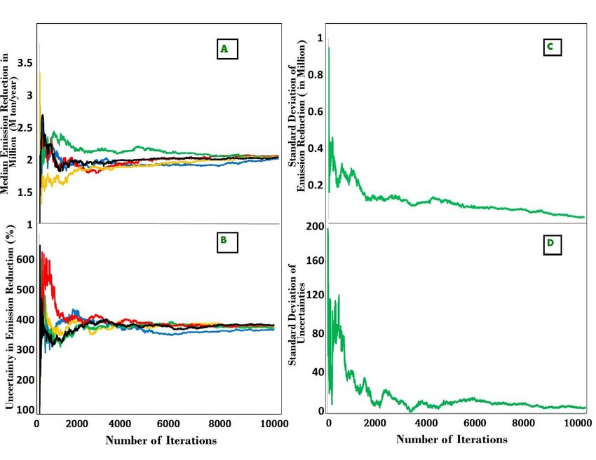
The # sign can be used in place of
 =NORM.INV(RANDARRAY) in simple formulas that
 do not sample from a distribution. The # copies the
 formula to fill the array. This is useful for
 calculations that do not require random sampling.

 This is effectively the same as the advantage of
 RANDARRAY, the formula needs to be typed only
 in the first cell, and it will autofill for every iteration.

Potential Pitfalls

If converted to a Google Sheet, all of the formulas using the # will have an error message called
ANCHOR ARRAY.

Using too few Monte Carlo iterations can provide imprecise uncertainty estimates. For your
emission reduction calculation, you can determine the number of Monte Carlo iterations needed
to achieve a desired confidence in your uncertainty estimates. In this example (based on the
Simple Example in Annex 1), uncertainty estimates are accurate to only about 20% of the
emission reduction even after 2000 iterations but approach 10% at 10,000 iterations (Figure
3.3).

 Figure 3.3. The similarity of Monte Carlo estimates depends on the number of iterations.

 13

a) Median of Monte Carlo estimates of the emission reductions, calculated for numbers of
 iterations up to 10,000 for 5 independent Monte Carlo runs.

 b) (b) The half width of the 90% CI of the Monte Carlo iterations divided by the median ER
 for the same 5 Monte Carlo runs.

 c) The standard deviation of the 5 Monte Carlo estimates of emission reductions.

 d) The standard deviation of the 5 Monte Carlo estimates of uncertainty.

3.4 How to interpret the output of the Monte Carlo

The Monte Carlo output can be analyzed to characterize the uncertainty in the results of the
calculation.

 1. Find the median (50th percentile) of the Monte Carlo outputs
 2. Find the 5th percentile of the outputs
 3. Find the 95th percentile of the outputs
 4. Calculate the half-width of the 90% confidence interval.
 5. Convert this to a percentage of the median.

 Spreadsheet Formula R Code

 Where Monte Carlo output is in cells B1:B10000 Considering a vector of simulated numbers
 SimNumC (c1,c2,c3,...,cn):

 A1 =MEDIAN(B1:B10000)
 A1

Step 4. Evaluate the contribution of each source to the overall
uncertainty
Understanding how much uncertainty is contributed by each source will help to identify
opportunities for reducing uncertainties. Evaluating the overall uncertainty with different inputs
assumed to be perfectly known is one way of assessing the sensitivity of the overall uncertainty
to uncertainty in each input.
Conducting a sensitivity analysis is facilitated by switches for each input that turn the associated
uncertainty on or off. The overall uncertainty can be calculated with different combinations of
switches turned on, rather than changing the formulae in the Excel file or the code in R.

 Spreadsheet Formula R Code

 This is accomplished with an “IF” statement The code relevant to an uncertainty source can be
 referencing a cell used to switch a source “on” or activated using an “if” statement.
 “off” for the sensitivity analysis.

 For example, if cell A5 on the results page has the
 value “on” or “off”, and cell B5 on the inputs page
 has
 IF(‘resultspage’A5=”on”, 1, 0.0000000001)

 Each iteration of a random draw for the source is
 multiplied by cell B5. If the uncertainty source is
 “off”, 0.0000000001 is used instead of 0 to avoid
 errors in the NORM.INV function.

Comparing the importance of uncertainty in the various inputs can be accomplished by
evaluating each one alone, with all other uncertainties turned off, or by removing each one, with
all other sources turned on. From the point of view of evaluating the benefit of reducing a
particular source in the context of all the others, it is more relevant to report how much
uncertainty is reduced by eliminating that source than to report how much that source
contributes alone, and this is the approach recommended in the FCPF Guidelines on the
Application of the Methodological Framework. However, it is easier to understand the results of
considering one source at a time. And if there is a need to revise one source,

The following table shows the results of a sensitivity analysis of the Simple Example provided in
the Annex.

 Sources included Uncertainty Uncertainty
 (Megatons C/year) (% of Emissions)

 Reference Crediting ER Reference Crediting ER
 Level Level
 Period Period

 15

R:S 2.80 2.50 0.29 17 17 17

 CF 0.58 0.52 0.07 4 4 4

 Sampling uncertainty 3.29 2.95 0.36 21 21 21
 in EF

 Emission factors 4.44 3.98 0.46 27 27 27
 (from the above 3
 sources)

 Activity data 4.10 7.20 8.07 25 49 472

 All sources 6.09 8.54 8.46 37 58 492

In this example, uncertainties are high relative to the emission reduction. This is because in this
example the reduction in emissions was small (1.7 megatons C/year, see Fig. 4.1 for a
graphical explanation).

 Figure 4.1. (a) Uncertainties are 37% of reference level emissions and 57% of the monitoring
 period emissions. (b) Because the emission reduction is small, the combined uncertainty is a
 large fraction of the emission reduction (>400%).

 16

As shown in figure 4.2, uncertainties relative to the emission reduction will become smaller over
time if the emission reduction increases over time, assuming that the contributing uncertainties
are relatively constant over time (Neeff 2021).

 Figure 4.2. Uncertainty in estimating emission reductions by scenarios of effectiveness in
 reducing emissions below the reference level and by uncertainty in measuring emissions (from
 Neff (2021), modified from FAO 2019)

Potential Pitfalls
If uncertainty estimates are not very accurate (based on a small number of Monte Carlo
iterations), then by random variation, the uncertainty with a source turned off can be slightly
higher than with the source turned on. Reporting each source turned on, rather than each
source turned off, will avoid this problem. Increasing the number of Monte Carlo iterations
makes the uncertainty estimates more precise (Figure 3.3).

 17

Literature Cited
Efron, B., Tibshirani, R. J. 1994. An introduction to the bootstrap. CRC press.
 FCPF 2016. Carbon fund methodological framework. Forest Carbon Partnership Fund
 Report.
 Available at: https://www.forestcarbonpartnership.org/system/files/documents/FCPF
 %20Carbon%20Fund%20Methodological%20Framework%20revised%202016_1.pdf
FCPF 2020. Guidelines on the application of the Methodological Framework Number 4 On
 Uncertainty Analysis of Emission Reductions. Forest Carbon Partnership Fund. Forest
 Carbon Partnership Facility Report. Available at:
 https://www.forestcarbonpartnership.org/sites/fcp/files/FCPF%20Guidelines%20on%20
 Uncertainty%20Analysis_2020_0.pdf
IPCC 2006. IPCC guidelines for national greenhouse gas inventories. vol. 4 agriculture, forestry
 and other land use. Prepared by the National Greenhouse Gas Inventories Programme.
 S Eggleston, L Buendia, K Miwa, T Ngaraand K Tanabe. Institute for Global
 Environmental Strategies, Hayama, Japan. Available at: https://www.ipcc-
 nggip.iges.or.jp/public/2006gl/vol4.html
IPCC 2019. Refinement to the 2006 IPCC guidelines for national greenhouse gas inventories.
 Prepared by the National Greenhouse Gas Inventories Programme. G. Domke, A.
 Brandon, R, Diaz-Lasco, S. Federici, E. Garcia-Apaza, G. Grassi, et al. Institute for
 Global Environmental Strategies, Hayama, Japan. Available at: https://www.ipcc-
 nggip.iges.or.jp/public/2019rf/vol4.html
Neeff, T. What is the risk of overestimating emission reductions from forests – and what can be
 done about it?. Climatic Change 166, 26 (2021). https://doi.org/10.1007/s10584-021-
 03079-z
Pistilli, Tony. “Behind the models: cholesky decomposition.” Medium, Towards Data Science, 23
 May 2019, towardsdatascience.com/behind-the-models-cholesky-
 decomposition-b61ef17a65fb.
 Zaiontz, C. 2020. “Cholesky Decomposition”. Real Statistics Using Excel, www.real-
 statistics.com/linear-algebra-matrix-topics/cholesky-decomposition/.

 18

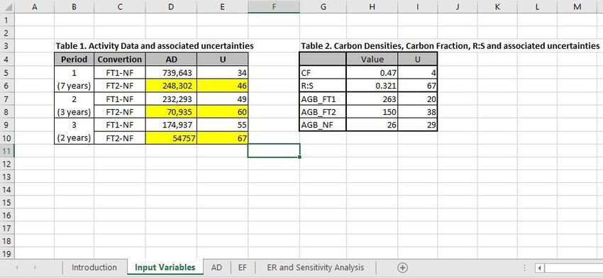
Annex 1. Monte Carlo Example in Excel
The simple example in Excel has two versions, one with a 2-year crediting period, and one with
a 4-year crediting period, which illustrates the high uncertainty associated with a short crediting
period.

Two forest types are included in the simple example, and deforestation is the only land-use
transition. The example illustrates a deforestation rate of 3% per year in both forest types.

Introduction
The first sheet of the Excel workbook describes the roles of the subsequent sheets.

Input Variables

The Input Variables sheet has all the data needed for the calculation of emission reductions.
Table 1 is activity data, or the . area of land converted from forest type 1 to non forest (FT1-
NF) and the area of land converted from forest type 2 to non forest ( FT2-NF) for the total 10
year time period: seven years of reference period and three years of monitoring period. Table 2
has emission factors including carbon fraction (CF), root to shoot ratio (R:S), and above ground
biomass (AGB).

Uncertainties are given as the half width of the 90% CI. The SE is calculated from the
uncertainty and the value of the estimate, although we recognize that in reality, the uncertainty
is calculated from the SE.

 19

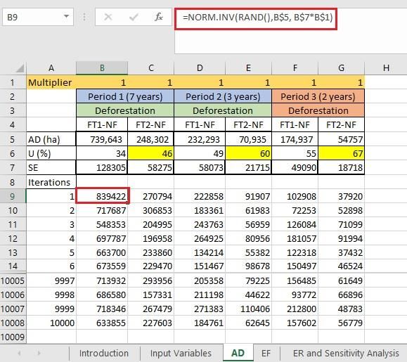
Activity Data (AD)

In the Activity Data sheet, forest transition data for each time period are simulated using Monte
Carlo Simulation as: =NORM.INV(RAND(), B$5, B$7*B$1)

 NORM.INV(probability, mean, sd) gives an inverse of the normal cumulative
 distribution, at the specified probability, mean, and standard deviation (sd).

 RAND() generates uniform random normal values between 0-1.

 B$5 is the mean of the value.

 B$7 is the standard error.

 B$1 is a multiplier controlled by a switch in the ER and Sensitivity Analysis sheet.

 20

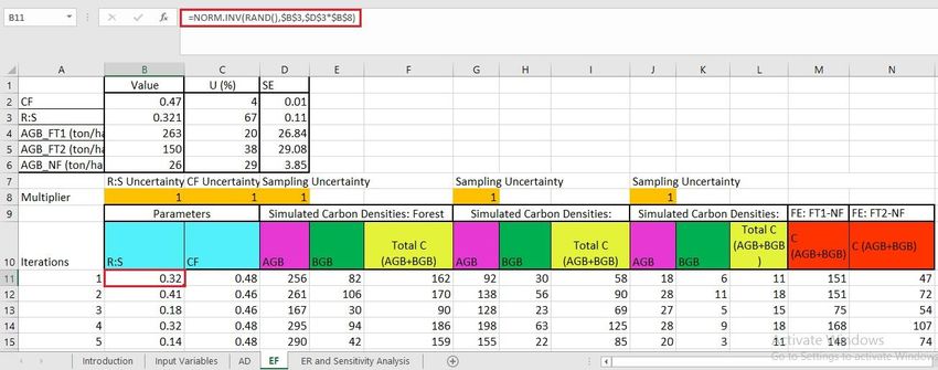
Emission Factors (EF)

In the Emission Factor Sheet, R:S, CF and AGB for each forest type are simulated using Monte
Carlo simulation.

Belowground biomass (BGB) is calculated by multiplying each simulated AGB value with the
simulated R:S value.

Total carbon for each land cover type is calculated as the sum of AGB and BGB.

Emission Factors (EF) are calculated as the difference in total carbon between land cover
types. Column M depicts the transition from forest type 1 (FT1) to non forest (NF). The process
is repeated for FT2-NF in column N.

The cells below row 10 are simulated values for each input variable. Multipliers in row 8 are
controlled by switches on the ER and Sensitivity Analysis sheet.

 21

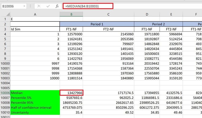
ER and Simulation

Emissions for each forest transition are calculated by multiplying Activity Data (AD) from the AD
sheet by Emission Factors (EF) in the EF sheet.

 1. In row 10006, the median of all simulations for each forest type is calculated as

 =MEDIAN(B4:B10003)

 2. In row 10007, the 5% percentile of all simulations for each forest type is calculated as

 22

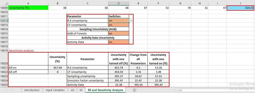
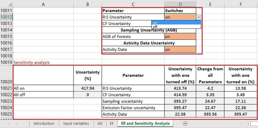
=PERCENTILE(B4:B10003, 0.05)

 3. In row 10008, the 95% percentile of all simulations for each forest type is calculated as

 =PERCENTILE(B4:B10003, 0.95)

 4. In row 10009, the half width of the 90% confidence interval is calculated as: (95
 percentile-5 percentile)/2

 i.e. (B10008-B10007)/2

 5. Finally in row 10010, uncertainty is calculated as: (half of 90% confidence
 interval/median)*100

 i.e. (B10009/B10006)*100

Switches

In the image below, the final uncertainty of Emission Reductions (cell X10009) is highlighted in
blue. When the switches in cells D10012:D10017 are ‘on’ the related multipliers are set to 1.
When the switches are ‘off’, the multipliers are set to 0 (or 1E-10, which is close to 0, and avoids
errors in the excel formula). The uncertainties change slightly every time the workbook updates
and the random values are resampled.

 23

This image depicts what happens when R:S uncertainty is turned off in the EF tab.

The contribution of each source to the overall uncertainty can be determined by starting with all
sources on and turning off each source one by one, or by starting with all sources off and
turning them on one by one. The sensitivity analysis table is populated with the values copied
from cell J1009 with different combinations of switches on or off.

 24

25

Annex 2. Monte Carlo Example in R

https://github.com/mark78b/MCS_in_R/

The Simple Example in R is the same as that in Excel, showing deforestation rates of two forest
types.

 1. Library loading
 To run the current R code, load the following libraries:

 library(matrixStats)
 library(gridExtra)
 library(reshape)

 2. Reading of inputs by Forest Type and Period
 Read the specific values of AD and EF (and associated uncertainties) by Forest Type (FT) and
 Period (P). Read csv Tables of AD and EF as follows:

 rm(list=ls(all=TRUE))

 ### Address to read inputs
 setwd("C:/Desktop/Inputs”)

 ### Reading of inputs
 # AD inputs
 BaseAD

and EF estimators. Nevertheless, in most cases, only uncertainties of AD and EF are reported.
 So it is necessary to compute SE of AD and EF as following:

 1/2 1.96 ̂
 = 100 ⇒ = 100 ⇒ =
 ̂ ̂ 1.96 100

 U = uncertainty
 IC= confidence Interval
 = estimator of AD or EF
 = standard deviation

 Once SE of AD and EF have been computed, it is possible (i) to generate vectors of random
 numbers of AD and EF per FT-P, (ii) to estimate emissions per FT, and (iii) to save vectors of
 simulated emissions by FT in matrix format.

 Following is show how to simulate random numbers (of normal distribution, using mean and
 standard error) of independient AD and partially correlated EF:

 #################### 1. Simulation of Activity Data ###################

 #### Computing of SD of AD
 BaseAD$DesEstDA

Matrix_AD

Matrix_EF$C_FT2

5. Estimation of quantiles and uncertainties
 Using vectors of simulated emissions it is possible to estimate associated lower/upper
 uncertainties as follows:

U_inf= Uncertainty on the left side of the simulated emissions

U_sup= Uncertainty on the right side of the simulated emissions

Q (0.025)= quantile 0.025 of simulated emissions

Q (0.975)= quantile 0.975 of simulated emissions

 = Monte Carlo simulated emissions

 (i) so, lower/upper quantiles of Base Line emissions can be estimated as:
 Q_05_FREL

Finally, probability density functions (PDF) of emissions by period and for median emissions are
 plotted:

 ### Saving of PDF of Base Line emissions
 setwd("C:/Users/Invited/Outputs")

 pdf("1_Emissions_Uncertainty_FREL.pdf")
 par(mfrow=c(2,1))
 hist(Table_Emi_FREL$FREL,
 main="Histogram of FREL",
 xlab="Average annual emissions from deforestation (Ton of CO2e)",
 cex.lab=1, cex.axis=0.8, cex.main=1,
 #border="blue",
 col="green",
 las=1,
 breaks = 200,
 prob = TRUE)
 lines(density(Table_Emi_FREL$FREL ))
 dev.off()

A draft version of the R code shown above is available at the following link:
https://github.com/mark78b/MCS_in_R/

 31

Document information

 Version Date Description

 1.0 21 September 2021 Initial version

 32