Climate-Change Profiles for the Capital Region of Bogotá-Cundinamarca, Colombia

Con la colaboración de:

 Plan Regional Integral de Cambio Climático Región Capital, Bogotá – Cundinamarca
                               PRICC Región Capital

        Climate-Change Profiles for the Capital Region of Bogotá-
                      Cundinamarca, Colombia
      Summary of initial procedures undertaken to develop scenarios of climate change
                               Michael J. Puma, Mark Tadross

This short report summarizes initial efforts at formulating climate-change scenarios for the
capital region of Bogotá-Cundinamarca, Colombia, as part of a collaborative effort between the
United Nations Development Programme (UNDP) and Colombia’s Institute of Hydrology,
Meteorology and Environmental Studies (IDEAM) within the project ’Plan Regional Integral de
Cambio Climático Región Capital, Bogotá-Cundinamarca’. The overall approach for climate-
scenario development is based on methods described in the UNDP publication entitled
Formulating Climate Change Scenarios to Inform Climate-Resilient Development Strategies: A
Guidebook for Practitioners [Puma and Gold, 2011] – an approach designed to help guide
decision makers’ through the following stepwise process:

       Step 1: Assess reasons and uses for climate-scenario development
       Step 2: Identify constraints to climate-scenario development (e.g. financial, computing,
       workforce, scientific) and determine needs for climate-scenario development in light of
       constraints
       Step 3: Evaluate existing approaches to generate a prospective range of climate
       scenarios against identified needs, and build a strong team
       Step 4: Develop and document climate scenarios

IDEAM and UNDP team members worked through this approach to develop climate scenarios
for the Bogotá-Cundinamarca region. Here, we briefly describe the specifics of how climate
scenarios were prepared, as well as some of the important problems and barriers that were
encountered along the way, so that future efforts for other Colombian regions can benefit from
these experiences.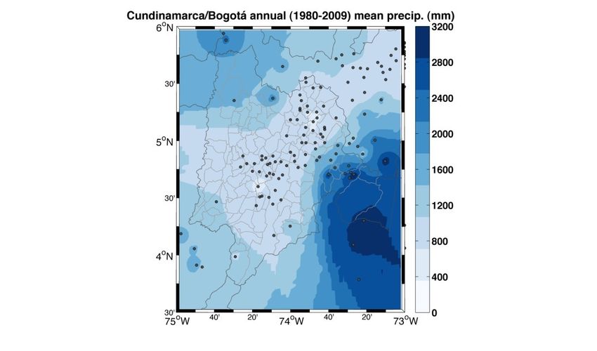

Step 1: Why were climate scenarios needed?

As part of Step 1, team members had general discussions on the potential uses of the climate-
scenario information. Discussions revealed that climate scenarios are needed for decision-
making at the municipal level. Mean climate variables (temperature, precipitation) and their
future changes over the next 10-, 20-, and 30-year horizons are needed to support municipal
decision making in several sectors, including water resources, forestry, agriculture, ecosystems
and energy. Beyond mean climate variables for different time horizons, a clear need for
information on the current and future extremes of temperature and precipitation was also
identified.

Implications for future work

Team discussions were valuable in terms of identifying the general use of the climate
information, which has allowed the team to generate, to some extent, climate scenarios at
appropriate spatial and temporal sales. Moving forward, however, more specific information
on the application of these climate scenarios would help to better focus their development.
That is, if further discussions can help identify the climate-related decisions that municipal
leaders need to make, then more detailed and relevant climate information can be generated.
For example, the climate information required by municipal leaders will differ depending on
what sectors (e.g. agriculture, water resources, health etc.) or climate hazards (high intensity
rainfall, start of the rains, seasonal duration etc.) they are planning for. These discussions are
also crucial for the analyses of extremes currently underway. Furthermore, a clear focus from
these discussions can help streamline the preparation of climate scenarios, improving the
efficiency and relevance of climate-scenario-development efforts.

Step 2: What were the major constraints?

Personnel and time constraints were a major consideration during the initial stages of our
efforts to develop climate scenarios. Limited personnel (1 climate scientist, on a part-time
basis, with support from IDEAM) were available to work on the climate-scenario development
for 2 to 3 months. Related to these personnel and time constraints was the issue of data
access. Quality controlled and gap-filled data were not readily available to develop a baseline
climatology for the region. Thus, IDEAM team members needed to devote efforts to data
preparation from the numerous meteorological stations. Considering that a significant amount
of time was needed to prepare the baseline climate information, limited time was available to
compute and analyze future climate scenarios. The method for prediction of future climate
conditions therefore needed to be a time-efficient approach that matched the personnel and
time constraints of the project. New analyses currently underway (focusing on extremes) will
potentially benefit from additional personnel and time, with new team members available both
at UNDP and IDEAM.

Steps 3 and 4: What were our options and how did we proceed?

The next task was to select a specific approach for climate-scenario development that was
consistent with the available resources for the analyses. We needed to decide what
downscaling approach would be used to combine the baseline climate data with projections of
future climate change available from global climate models. The general options include basic
downscaling, statistical downscaling, and dynamical downscaling. Of these three, dynamical
downscaling is the most time intensive, so no new dynamical downscaling could be done.
However, we did have access to some limited dynamical downscaling results from PRECIS
(http://www.metoffice.gov.uk/precis/intro), the Hadley Centre's regional climate modeling
system, for the Bogotá-Cundinamarca region. We did some initial assessment of the PRECIS
climate change predictions, but decided not to use these model data for our primary climate
scenarios (though they can be used to provide additional information if needed), because these
dynamically downscaled results were only available for 1 or 2 global climate models.

Standard GCM outputs and statistical downscaling, the other main options, can both be time
efficient, if the team has well developed and readily accessible tools. We selected the change-
factor methodology (CFM), a basic time-efficient approach, to develop climate scenarios. The
CFM was selected as an initial approach as it matched our time and financial capacity for the
project, allows the integration of predictions from many global climate models, and does not
require use of any specialize software – thereby making it an approach that can be readily
accessible to local researchers in Colombia. Statistical downscaling methods can be equally
efficient in terms of time and computational resources, which may be used for further analyses
in the region.

The CFM approach, as with most methods, consists of a historical climate analysis and future
climate projections. In the sections below, the three procedures used to develop these climate
scenarios for the Bogotá-Cundinamarca region are described, so that future efforts can clearly
build on this work.

Developing a station-based climatology (Procedure 1)

The first task was to obtain daily rainfall and temperature data from as many stations in
Bogotá-Cundinamarca and the surrounding districts as possible. The goal was to establish a
baseline climate for the region, with a focus on the period 1980 to 2009. We selected a 30-year
period, because averaging over a period of this length will take into account any decadal-scale
variability of temperature and precipitation that might exist in the region. The key challenge
was the discontinuous data of varying quality and spread non-uniformly over the region.

To prepare the meteorological station data for analyses, a quality control (QC) method needed
to be applied to the data. Data QC is essential, because our efforts to identify and understand
changes and variations of regional climate are very sensitive to erroneous data (due to
incorrect units and readings as well as typos). The QC methods were led by Team-member
Leon and are described in Appendix A.

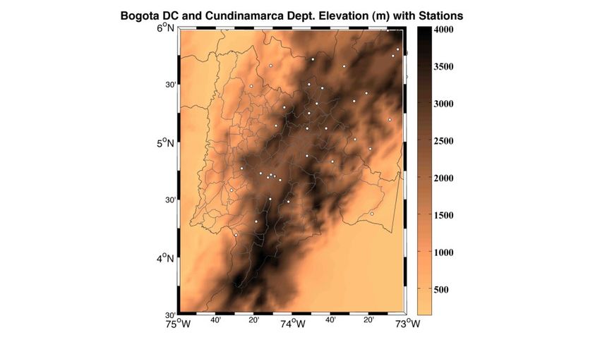
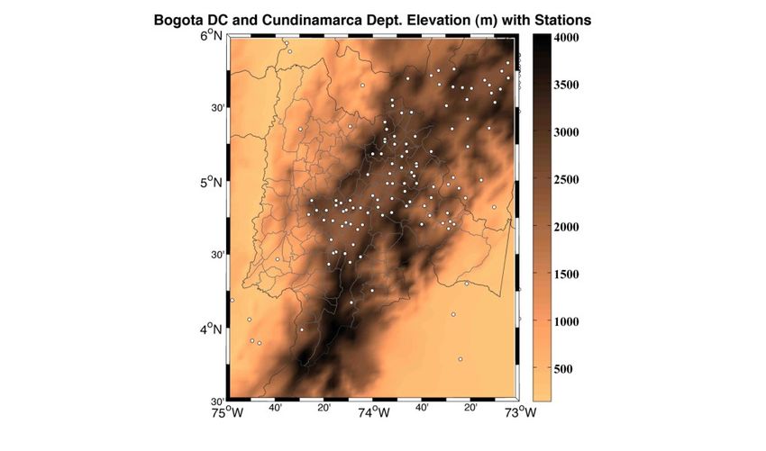
In conjunction with the QC efforts, time periods with missing data needed to be gap-filled. A
robust gap-filling method is needed, because a realistic and continuous dataset allows us to
compute an accurate climatology, including the average conditions, seasonality, and variability.
Continuous datasets are also essential for many applications, especially those related to water
resources. Team-member Leon’s dataset also led the gap-filling effort (Appendix A). There
was, however, an issue at many stations where too much of the data overall was synthetic and
that the synthetic values often led to a situation where we had too many consecutive days with
the same value. Team-member Puma visual inspected the station data to remove stations
where approximately 20% or more of the data were synthetic. Limited time prevented Team-
members Leon and Puma from applying more robust quality control and gap-filling procedures.
Coordinating better QC and gap-filling procedures must be a priority moving forward.

Figure 1: Elevation and station locations for (left) temperature and (right) precipitation used in
the analyses.

The next task was to interpolate the quality controlled and gap-filled station data. Two
interpolation methods were applied: ordinary kriging and the inverse distance weighting
method. Generally, the differences between the interpolated surfaces for each method were
relatively minor.

Elevation was a key factor for station-data interpolation in Bogotá-Cundinamarca. Previous
experience and our data analyses demonstrated that temperature is strongly dependent on
elevation. The relationship between precipitation and elevation was much less clear, likely due
to the complex topography in the region. Therefore, we interpolated assuming temperature is
dependent on elevation while precipitation is independent of elevation.

Many options exist for including a dependence of temperature on elevation. Dodson and
Marks (1997) describe a relatively straightforward approach, which is used here. These authors

used a neutral stability model to account for elevation dependence, which involves three main
steps:
   1. Convert air temperatures to potential temperatures (Equation 1 of Dodson and Marks,
       1997). To compute the potential temperatures, an estimate of the pressure at each
       station is needed.      The station’s elevation, along with a form of the hydrostatic
       equation, allows us to compute these pressures.
   2. Spatially interpolate points the potential temperatures to a grid surface using the IDW
       method. The digital elevation map (DEM) in the next step determines the resolution of
       the grid surface.
   3. Use the inverse of the potential temperature function to map the surface to DEM
       elevations. The DEM files were from ETOPO2v2 Global Gridded 2-minute Database,
       which has a horizontal resolution of 2 decimal minutes and a vertical resolution of 1
       meter. The dataset is available from the National Geophysical Data Center of the
       National Oceanic and Atmospheric Administration (U.S. Department of Commerce) at
        http://www.ngdc.noaa.gov/mgg/global/etopo2.html.

This approach was applied to the temperature data from 41 stations in Bogotá-Cundinamarca
and its surroundings. The spatial resolution of the interpolation was chosen to be 5 km (i.e. 5
km by 5 km grid boxes), which was obtained using IDW method using only horizontal distances
in the second step above. For precipitation, inverse distance weighting interpolation was
applied directly to the quality controlled and gapfilled dataset; many more stations were
available for this (133 stations) compared to the relatively small number available for
temperature.

It is important to note that the spatial scale at which we can interpret the interpolated variables
depends very much on the station density as well as the characteristic spatial scales associated
with the regional heterogeneity of temperature and precipitation. In Figure 1, we can see that
few stations are present in the western and southern portion of Cundinamarca. The
consequences of this sparse density of stations significantly affected the interpolated
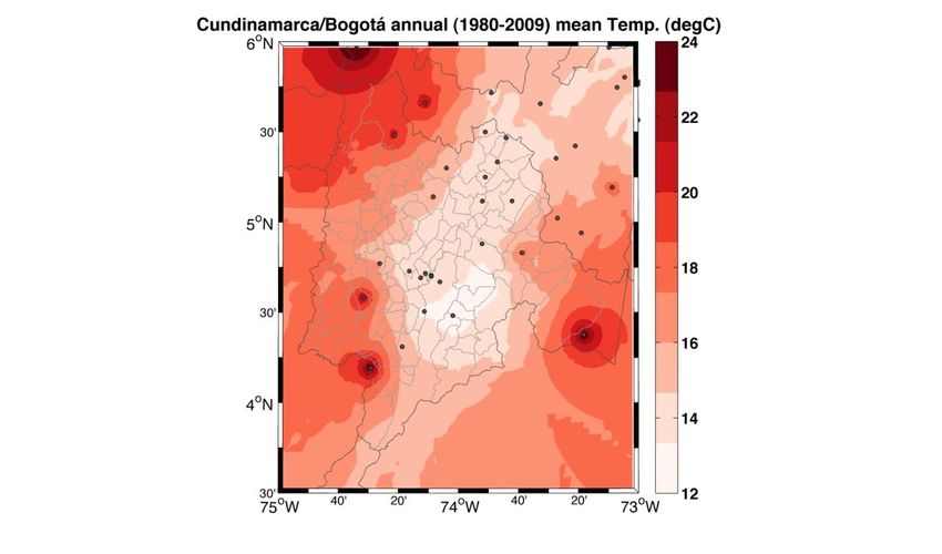
temperature surfaces in the western and southern portions of Cundinamarca as shown in the
left panel of Figure 2. Although there are clearly more stations with precipitation data, station
density still appears to be an issue in Cundinamarca’s western sections (Figure 2, right panel).
As the results of these analyses are shared with municipal-level decision makers, it is essential
to point out these issues.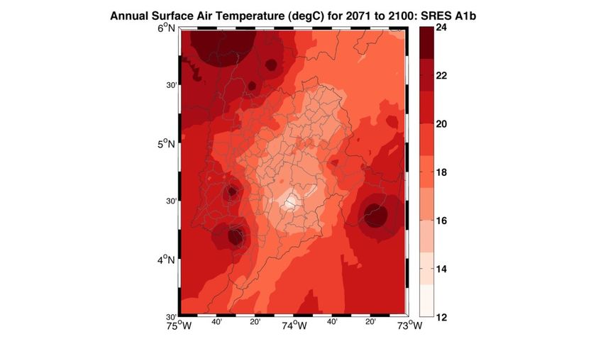

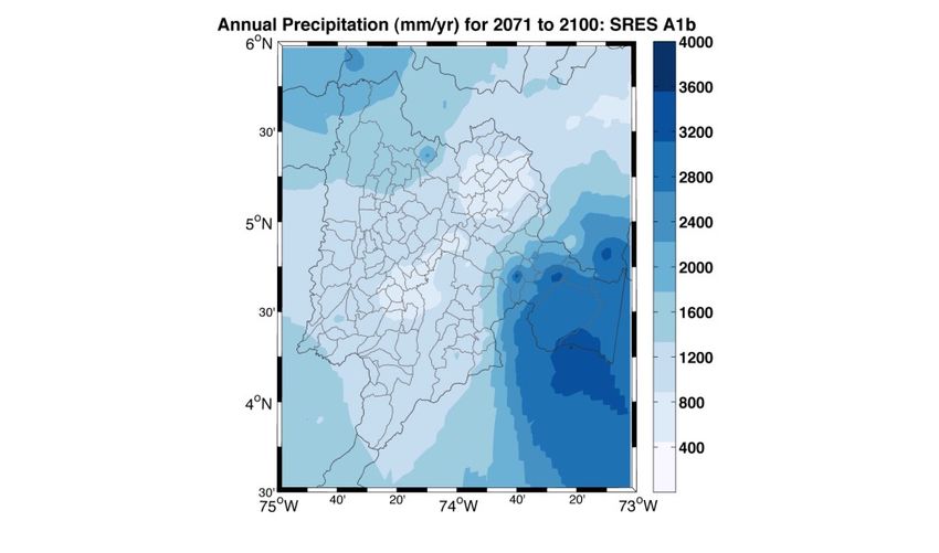
Figure 2: Interpolated annual (right) temperature and (left) precipitation data for the region
using the inverse distance weighting method.

Lessons learned

During this process, there was a clear need for a standard and robust procedure for quality
control (QC) and gap-filling of data. Efforts are currently underway to identify a procedure that
can be applied to the analyses of temperature and precipitation extremes as well as to similar
analyses for other Colombian Departments. Potential gap-filling methods include the
procedures of Teegavarapu and Chandramoul [2005]. Potential QC approaches include those
of Feng et al. [2004] and You et al., [2007]. However, the effort required for implementation of
these procedures needs to be weighed against how they may affect the underlying data and
therefore the information that is derived from it. For example, if too much missing data is
replaced with the average (or climatological) values then the variability of the time series will
be reduced, affecting the significance and magnitude of calculated trends. As we conduct these
analyses, it is clearly beneficial to include as many stations as possible, including those in
Departments surrounding the region of interest (as these are needed for more accurate
interpolation towards the edge of the Department). Considering this, in the future it would be
more efficient to prepare a climatology for the entire country at once rather than duplicating
efforts when going Department by Department.

Compute a model-based change between present and future climate using GCMs (Procedure
2)

Global climate models (GCMs) were used to quantify how temperature and precipitation will
change from the present-day climate. In this procedure, the difference (anomaly) between the
current and future climate was computed based on GCM output. The mean current (baseline)
climate is computed as

Nb

                                                ∑ GCM      b,i
                                                i=1
                                      GCM b =
                                                 Nb
where GCMb,i is the value of the baseline GCM variable (e.g. temperature, precipitation) for
time period i and Nb is the number of values (i.e. number of years) for the baseline period.
Analogously, the mean future climate is computed as
                                                Nf

                                                ∑ GCM      f ,i
                                                i=1
                                      GCM f =
                                                      Nf
GCMf,i is the value of the future GCM variable for time period i and Nf is the number of values.

The GCM output for current and future climate is used in different ways, depending on the
variable of interest. For temperature, an additive change factor is computed as
                                    CFadd = GCM f ,i − GCMb,i
where CFadd is the additive change factor. This difference is then added to the locally observed
values in the procedure that follows. The underlying assumption is that a GCM is skillful in
estimating the absolution chance in a climate variable, regardless of the GCM’s accuracy in
predicting current climate [e.g., Anandhi et al., 2011]. The multiplicative change factor,
commonly used for precipitation, differs from the additive change factor in that the ratio
between the future and current climate is computed, which is expressed as:
                                     CFmul = GCM f ,i GCMb,i
where CFmul is the multiplicative change factor. The locally observed values are then multiplied
by this factor in the procedure that follows. When this change factor is used, the inherit
assumption it that the GCM is skillful in estimating the relative change of a climate variable
[e.g., Anandhi et al., 2011].

Developing future scenarios (Procedure 3)

In this procedure we obtain local scaled future values by applying CFadd and Cfmul to the
observed baseline from Procedure 1. The future temperature values are computed using the
additive change factor as
                                       LOf ,i = LOb,i + CFadd
while the future precipitation values are computed as
                                        LOf ,i = LOb,i ⋅ CFmul
where LOb,i and LOf,i are observed and future values, respectively, of the meteorological
variable for time period i at a grid point. These calculations are applied to the monthly GCM
data. LSf , add, i = LO b, i + CFadd

Selecting GCMs, emissions scenarios, and future periods

The procedures described above can be applied to one or more GCMs as well as one or more
greenhouse gas (GHG) emissions scenarios. We selected GCMs for the analysis based on the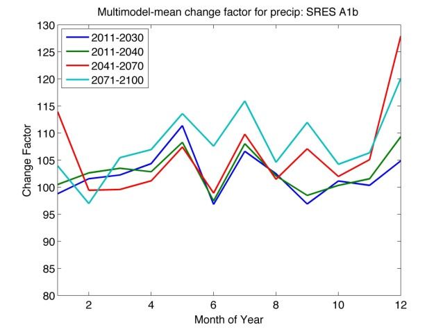

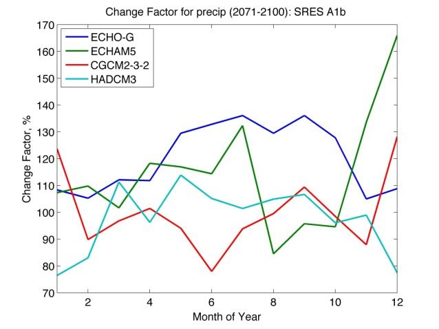
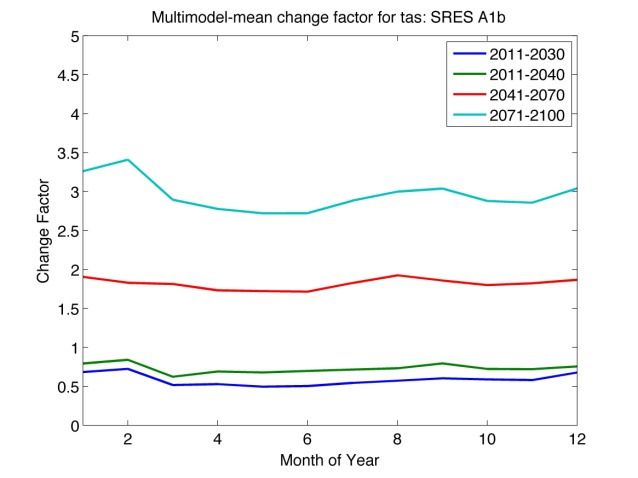
results of Rodríguez Roa [2010]. In this report, four GCMs were identified to be most skillful at
simulating present-day climate for Colombia based on multiple criteria. The following GCMs
were identified as most skillful based on evaluation of their output available in the World
Climate Research Programme (WCRP) Coupled Model Intercomparison Project Phase 3 (CMIP3)
multimodel dataset:

   1.   ECHO-G
   2.   MPIECH-5: ECHAM5/MPI-OM
   3.   MRI-232A: MRI-CGCM2.3.2
   4.   UKHADCM3: HADCM3

Three GHG emissions scenarios were selected to provide a bounding range of predictions and
an assumed ‘middle-of-the-road’ scenario. The scenarios were based on the widely used
Special Report on Emissions Scenarios (SRES) scenarios, where the upper and lower bounding
scenarios were A2 and B1, respectively, and the middle-of-the-road’ scenario was B1. The
future periods of interest in this analysis, as identified by the Colombian team, were 2011 to
2030, 2011 to 2040, 2041 to 2070, and 2071 to 2100. These periods were selected to match
time periods from other climate-related projects currently underway in Colombia.

Figure 3: Monthly change factor for (right) temperature and (left) precipitation computed using
the ECHO-G, ECHAM5/MPI-OM, CGCM2.3.2, and HADCM3 global climate models for the period
2071 to 2100 and SRES scenario A1b.

As an example, Figure 3 shows the monthly change factors for both temperature and
precipitation for the four GCMs. Interesting, there is significant spread in the changes for both
variables among these ‘best’ models. However, multimodel change factors were computed and
used in these analyses. These multimodel change factors are should in Figure 4. The annual
future climate scenario for SRES scenario A1b for the period 2071 to 2100 is shown in Figure 5.
The spatial patterns are maintained from the baseline climatology in Figure 2, because we are
applying the change factor uniformly in space and time.

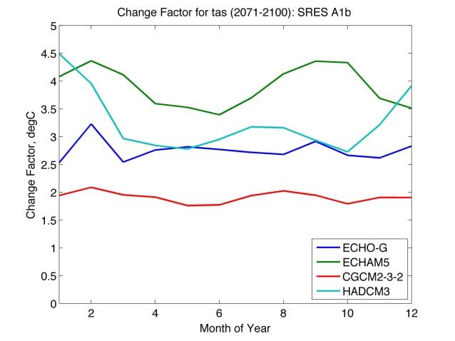
Figure 4: Monthly change factor (right) temperature and (left) precipitation data for the region
using the inverse distance weighting method.

Figure 5: Future climate scenarios for the period 2071 to 2100 for (right) temperature and (left)
precipitation using the change factor methodology based on 4 GCMs.

Additional analyses

Additional efforts are now underway to conduct analyses of extreme temperatures and
precipitation, using daily rainfall and temperature from both observations and statistically
downscaled data for Bogotá-Cundinamarca. These analyses will be conducted by a local
(Colombian) team member, Blanquita Oviedo, under the direction of Mark Tadross and with
additional support from Gloria Leon, Michael Puma and others. The main steps for these
additional analyses are outlined in Table 1.

Table 1: Key steps in developing downscaled future scenarios and observed trends in extreme
climate indices for Bogotá-Cundinamarca.

Key required steps                                  Output

Analysing historical trends
1. Obtain daily rainfall and temperature data for   Precipitation and temperature data for
as many stations in the district and surrounding    historical observations
districts: minimum of 10 years non-continuous
data post 1979 (for downscaling), minimum 30+
years data for trend analysis
2. Quality control data checking for missing        Quality controlled data
values, unrealistic rainfall and temperature
values
3. Reformat data into STARDEX and Rclimdex          Rainfall and temperature data for
formats, as well as UCT format                      historical observations
4. Apply STARDEX and Rclimdex software to           Historical time series of extreme indices
calculate annual and seasonal trends in extreme     available + calculated trends in those
climate indices                                     indices

Developing future climate scenarios
5. Apply GCM change factor to available             GCM estimates of monthly rainfall and
observations                                        surface temperature
6. Statistically downscale future climate for 7+    Statistically downscaled estimates of
GCMs for the A2 and B1 emissions scenario and       daily rainfall and temperature for a
2046-2065 period (done at UCT).                     range of GCMs available
7. Develop ways of visualising data - changes in    Figures and tables useful to understand
rainfall and temperature based on seasonal          what climate change will likely entail for
cycle, calculating changes in statistics,           a station/region
comparing models with observations etc.
8. Tailored data analysis based on user/policy      Depends on user feedback
requirements and thresholds of interest

The climate analyses presented here can be developed further (e.g. using improved baseline
climate data or enhanced change factor methods) or can be modified to use other available
data (from regional climate models) or approaches (e.g. statistical downscaling methods
developed at the University of Cape Town). Further discussions are also needed on whether to
include more GCMs as part of the analyses, so as to better categorise the likelihood of
simulated changes and associated risks. Also, the teams should consider whether to use newer
GCM output from the CMIP5 archives.

Acknowledgements

We wish to acknowledge the modelling groups, the Program for Climate Model Diagnosis and
Intercomparison (PCMDI) and the WCRP's Working Group on Coupled Modelling (WGCM) for
their roles in making available the WCRP CMIP3 multi-model dataset. Support of this dataset is
provided by the Office of Science, U.S. Department of Energy.

References
Anandhi, A., et al. (2011), Examination of change factor methodologies for climate change
impact assessment, Water Resources Research, 47(3), W03501.

Feng, S., et al. (2004), Quality control of daily meteorological data in China, 1951-2000: a new
dataset, International Journal of Climatology, 24(7), 853-870.

Puma, M. J., and S. Gold (2011), Formulating Climate Change Scenarios to Inform Climate-
Resilient Development Strategies: A Guidebook for Practitioners, United Nations Development
Programme, New York, NY, USA.

Rodríguez Roa, A. (2010), Evaluación De Los Modelos Globales Del Clima Utilizados Para La

Generación De Escenarios De Cambio Climático Con El Clima Presente

En Colombia, Instituto de Hidrología, Meteorología y Estudios Ambientales - IDEAM

SUBDIRECCIÓN DE METEOROLOGÍA, Bogotá, D. C.,.

Teegavarapu, R. S. V., and V. Chandramouli (2005), Improved weighting methods, deterministic
and stochastic data-driven models for estimation of missing precipitation records, Journal of
Hydrology, 312(1-4), 191-206.

You, J., et al. (2007), Performance of quality assurance procedures on daily precipitation, J.
Atmos. Ocean. Technol., 24(5), 821-834.