Constrained Discrete Model Predictive Control of a Greenhouse Relative Humidity
←
→
Page content transcription
If your browser does not render page correctly, please read the page content below
E3S Web of Conferences 229, 01001 (2021)                                                               https://doi.org/10.1051/e3sconf/202122901001
ICCSRE’2020

            Constrained Discrete Model Predictive Control of a Greenhouse Relative
                                         Humidity

               Hafsa Hamidane1 , Samira El Faiz2 , Abdeslam Lachhab1 , Mohammed Guerbaoui1 and Abdelali
                                                       Ed-Dahhak1
                1 Modelling,Materials and Control of Systems Team, High School of Technology, Moulay Ismaı̈l University, Meknes,
                                                                   Morocco
            2 Energy and Sustainable Development Research Team, High School of Technology, Ibn Zohr University, Guelmim, Morocco

                                     hamidanehafsa@gmail.com, Selfaiz@yahoo.fr, Abd lachhab@yahoo.fr

           Keywords:       greenhouse, relative humidity, constrained linear system, model predictive control, yalmip, optimization

           Abstract:       In this paper, we present a Constrained Discete Model Predictive Control (CDMPC) strategy application for
                           relative humidity control. In this sense, and for our system inside humidity dynamics description, a green-
                           house prototype is engaged and a state space form which fits properly a set of collected data of the greenhouse
                           humidity dynamics is presented as mathematical model. This latest is used for the CDMPC starategy appli-
                           cation, which purpose is to select the best control moves based on an optimization procedure regarding the
                           constraints on the control. By the means of Matlab/ Simulink and Yalmip toolbox algorithms, numerical sim-
                           ulations were held to proove the effectiveness of the controller, garanteeing both the constraints feasibility and
                           system stability.

           1     INTRODUCTION                                                      In control theory application, Model Predictive
                                                                               Control (MPC) has been always considered as one
           Agricultural greenhouses industry is nowadays con-                  of the most emerging control technique. Due to its
           sidered as one of the most important and high-                      advantages, this strategy has been used in various in-
           tech structures of all agrifood industry. In fact                   dustrial and automation process control (Wang et al.,
           seeking agricultural biodiversity, sustainable, high-               2017) , for instance the greenhouses climate control
           performing and protectable yields, has led to a vari-               (Ding et al., 2018) and reference therein.
           ety of advanced technologies adoption such as highly                    Moreover, (MPC) is engaged in a large variety of
           controlled and smart greenhouses.                                   systems, the main reason of its utility is its simplicity
                The environmental parameter control indooor                    of use which makes it appicable for single, multivari-
           greenhouses has known a considerable attention in the               able, linear and nonlinear systems, and allows con-
           last few years (Moufid and Bennis, 2019). The main                  straints notion incorporation when synthesising the
           reasons for this increasing interest are mainly related             control law (Wang et al., 2018; Faiz and Benzaouia,
           to different factors one can cite agronomic and finan-              2019) and many others as well .
           cial ones.                                                              The problem treated in our framework, is related
                In fact, various are the methods that have been                to control task of the relative humidity under green-
           treated regarding the control design of the climatic                house, hence model predictive control is choosen as a
           conditions of the greenhouses, hence several scien-                 modern control strategy to overcome this problem
           tific reaserchers and teams have experienced this tech-                 The objectif of the control technique, is to calcu-
           niques to study and enhance greenhouses control out-                late an objective funnction over a finite horizon, while
           standing, we can cite: neuronal networks control                    satisfying the constraints on the control notion, us-
           (Mohamed and Hameed, 2018; Taki et al., 2016) pre-                  ing Yalmip optimization as a novel toolbox(Lofberg,
           dictive control (Gandhi and Thakker, 2020). In ad-                  2004) together with Simulink, which allows a certain
           dition to the fuzzy control(Xu et al., 2020; Guer-                  minimization regarding overheads and unwanted cal-
           baoui et al., 2013), optimal control (Lijun et al., 2018)           culations.
           and many other strategies that have been discussed in                   The remainder of the prensent paper is struc-
           many research articles.                                             tured as follows, In the second section the greenhouse

© The Authors, published by EDP Sciences. This is an open access article distributed under the terms of the Creative Commons Attribution License 4.0
(http://creativecommons.org/licenses/by/4.0/).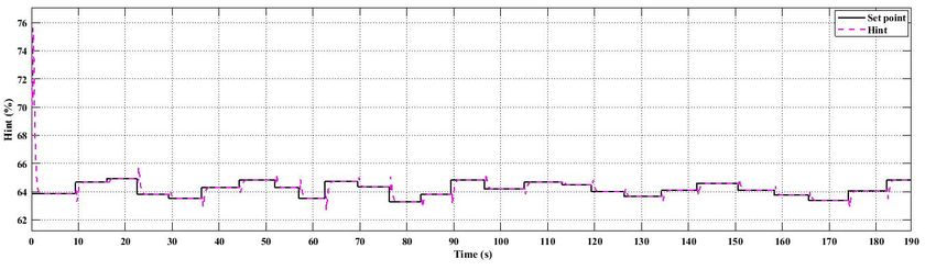
E3S Web of Conferences 229, 01001 (2021)                                                       https://doi.org/10.1051/e3sconf/202122901001
ICCSRE’2020

          model identification and a reminder of CDMPC pur-              2.2     Mathematical Modelling
          poses and controller strategy regarding the constraints
          notions, will be presented, in addition to the main            In this section, a mathematical model of indoor hu-
          control algorithm. The third section will be dedi-             midity has been presented. For this aim, the state
          cated to simulation results and discussion related to          space model that describes the greenhouse inside hu-
          the (CDMPC)design strategy and synthesis. In the               midity dynamic response to the installed actuators; is
          last section, some conclusions will be provided.               revealed. The adopted model will enable us to modify
                                                                         the behavior of the plant in order to suit our needs in
                                                                         term of reference signal tracking and control render-
                                                                         ing.
          2     MATERIALS AND METHODS                                        For controller synthesis and behavior aims, a plant
                                                                         model has to be obtained. Hence the system model
                                                                         is estimated by the means of collected data from the
          2.1    The Greenhouse System Prototype                         experimental greenhouse where the N4sid algorithm
                 Description                                             is used to identify the plant in discrete time state space
                                                                         model.
                                                                             For linear subspace identification and for simplic-
          In order to give an insight of our system, Figure 1
                                                                         ity, the class of systems to be considered is linear
          presents the experimental greenhouse engaged as sup-
                                                                         discrete-time systems with external disturbances of
          port in this work, which is a prototype installed at the
                                                                         the form:
          Laboratory of Electronics, Automatics and Biotech-
          nology (LEAB), Faculty of Sciences, Meknes, Mo-                              xk+1 = Axk + Buk + Kwk
                                                                                                                                (1)
          rocco. This system’s main construction is beeing a                              yk =             Cxk + Duk
          single wall polyethylene design, equipped with two             Where xk , uk , yk , wk present respectivelly the state,
          LM35DZ temperature sensors that provide indoor and             input, output and the output measurement noises vec-
          outdoor measurements of temperature and two HIH-               tors, A, B, C, D, K denote respectivelly the state, in-
          40 00-003 Honeywell indoor and outdoor relative hu-            put, output and estimated noise matrix.
          midity sensors. In addition, a heating system and a fan            As an advantage of the N4sid method, a prediction
          are installed to insure the appropriate climate for the        error based on a the Best Fit (BF) percentage related
          system’ s inside climatical environement. For con-             to the output reproduced by the model is provided,
                                                                         and the adopted formula used in this regard is pre-
                                                                         sented as follows (Carrión et al., 2011):
                                                                                                         |y − ŷ|
                                                                                      Best f it = (1 −            ) × 100      (2)
                                                                                                          y−y
                                                                         where y, ŷ and y are respectivelly the measured, the
                                                                         predicted model and the mean of the output y .

                                                                         2.3     Relative Humidity Response to
                                                                                 Actuators
                Figure 1: Experimental Greenhouse System.
                                                                         In this section, we aim to use a set of collected data in
          trol and data acquisition aims, the mentionned sensors         order to have the linear models that will be engaged
          and actuators are connected to a control and acquisi-          for mathematical identification.
          tion cards attached to a personal computer (Eddahhak
          et al., 2007). In the first place, an acquisition data         2.3.1   Relative humidity Response to heater
          card of the familly NI-PCI6024E from Advantech is
          installed to ensure the different actuator orders. Be-         Herein, we describe the evolution of indoor relative
          sides, two other cards are also installed and respec-          humidity by exciting the system with a step input of
          tivelly dedicated to the signals conditionning and the         2.5 Volts that was sent to the heater, till reaching a
          sensors as well as the hole system protection. In a            steady state. Using experimental data for 5 seconds
          second place; the tasks of supervision of measured             as sampe time and the N4sid algorithm under Mat-
          indoor and outdoor climate variables; are provided as          lab, the evolution of the measured and simulated in-
          a historical database using Labview, and the control           side relative humidity and the discrete time state space
          task is managed under Matlab/Simulink software.                model matrix are as follows.

                                                                     2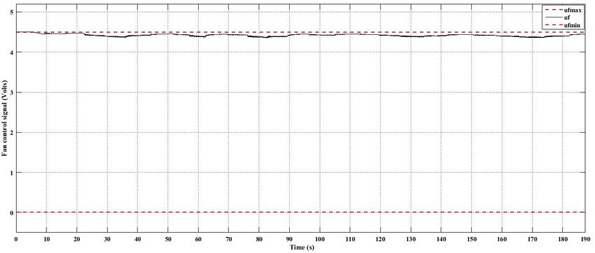
E3S Web of Conferences 229, 01001 (2021) https://doi.org/10.1051/e3sconf/202122901001
ICCSRE’2020
Figure 2: Comparison of Simulated and Experimental Figure 3: Comparison between Simulated and Experimen-
RHint Step Response to the heater tal RHint Step Response to the fan
As is shown, the inside humidity reaches 51%, As clearely shown, the indoor relative humidity
where the initial value is 71 to 74% . The model attends to reach its 72.3%, where the initial value is
best fit is 94%, hence the simulated and experimental 59%. The model best fit this time is 80.65 %.
resulting outputs are closely matching each other, The identified discrete-time system model, with 5
which is obviously seen from the fit accuracy.
Regarding the N4sid algorithm and “(1)”, the dis- states, was presented as follows:
crete linear time invariant system with 6 states is
−0.0669
definedned as follows: 0.9651 0.0564 0.0397 0.0134
0.0298
−0.08660 −0.8902 −0.6648 −0.4405
A f = −0.0430 0.6670 0.2978 0.1720 −0.2545
0.9899 −0.0145 −0.0030 −0.0065 −0.0083 0.0020 0.0030 0.0012 0.4613 −0.4973 −0.0767
0.0880 0.8398 −0.3343 −0.0669 −0.0429 −0.0572 0.0126 0.5068 −0.1236 −0.0854 −0.3511
−0.066 0.329 0.553 −0.493 −0.459 0.095 h iT
Ah = B f = −0.8393 −5.2316 −9.3999 11.9104 −7.8066
0.0026 0.0111 0.0041 −0.6158 0.7488 0.0910
0.0253 −0.0676 0.2400 −0.2388 0.0071 −0.8232
h i
C f = −35.0707 0.7589 −0.7247 −0.2962 0.1382
−0.0226 0.0999 −0.1911 0.2281 0.0762 −0.5882
Df = 0
h iT
Bh = −0.0010 0.0004 0.0433 −0.0643 −0.1262 0.1721 h iT
K f = −0.0199 −0.0055 −0.0117 0.0427 0.0217
h iT
Ch = 2.0057 6.5409 3.2425 2.0265 0.0672 0.1458
Under the initial state:
Dh = 0 h iT
x f 0 = −0.9173 6.4773 −45.4115 26.7665 −23.9029
h iT
Kh = 0.0019 0.0123 0.0111 −0.0429 0.0179 −0.0286
And the open-loop eigen values:
Under the initial state:
σ(A f ) = {0.9699, −0.6736, 0.0163, 0.0080 ± 0.8330i}
h iT
xh0 = 1.0376 −0.7908 0.6261 −0.4653 −0.4122 0.2439
The index ’f’ denotes the fan as input actuator
And the open-loop eigen values: used in the system state space identification.
The identified state space models, show that the
σ(Ah ) = {0.9839, −0.8857, 0.5102 ± 0.3542i 0.0340 ± 0.3468i} system is stable, controllable and observable.
The index ’h’ refers to the heater as first actuator
for the system state space identification. 2.4 The Control Task
2.3.2 Relative humidity Response to the fan 2.4.1 Brief Remainder of Constrainded (MPC)
and Optimization Problem Principles
Similarly, we excite the system with a step input of
2.6 Volts that was sent to the fan, in order to visualise Model Predictive Control, is an iterative finite horizon
the indoor relative humidity evolution, we notice; for control strategy, based on an optimization problem of
the same sample time, which is 5 seconds; that the a difinite plant model(Santana et al., 2020). Its main
humidity increases reaching by that a steady state. In task is that it allows a cost function calculation to ob-
this case, the evolution of the measured and simulated tain the performances of the controller in the future
inside humidity is depicted in “Fig. 3” : based on the current real or estimated plant state xk
3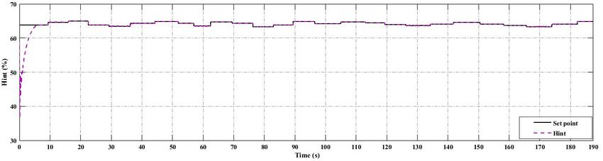
E3S Web of Conferences 229, 01001 (2021)                                                       https://doi.org/10.1051/e3sconf/202122901001
ICCSRE’2020

          and a serie of future inputs uk at each discrete sam-
          pling time (k).
              Due to their importance, the optimization task
          and the cost function are primordial in predictive
          control strategy, hence their contribution allows the
          calculation of the best series of control inputs uk ,
          which results in a minimal cost to keep the reference
          good tracking. For the control purposes, having a
          cost that describes how our control strategy will be
          in the future is the most important task to take into             Figure 4: Conceptual model of the CDMPC strategy
          consideration. Therefore, a function is adopted as
          follows (3):
                                                                         Where the suffix “min” and “max” are the lower and
                                J = f (xk , uk )             (3)         upper inputs constraints.
          Where xk and uk are the current state and control in-
          put, respectivelly. In order to get an optimal inputs          2.4.3   The Adopted Controller
          sequence u∗k , the cost function of uk has to be mini-
          mized, hence an optimal control problem is defined
                                                                         The control strategy used in this framework is a
          as follows:
                                                                         (CDMPC) formulation for greenhouse humidity con-
                          u∗k = arg min J(xk , uk )          (4)
                                  u                                      trol, it is presented as a Quadratic Programming (QP)
              The integration of the cost function (4), is chosen        problem solved at each sample time. The general
          to be quadratically dependent on the control input and         and conceptual presentaion of the control method is
          the state or output. In this sense, an optimization pro-       depicted in figure 4 In addition, the constraint on
          plem cost function of the form (5), is calculated.             the control notion regarding the system dynamics is
                                                                         brought into the cost function for MPC formulations.
                                       N                                 This latest will penalize any deviation regarding the
                   minimize J =
                        u
                                      ∑ xk0 Qxk + u0k Ruk     (5)        systems output which is the inside humidity; and the
                                      k=1                                input as well trying to have the optimal control se-
          Here N, Q and R represent respectively the prediction          quence. The constrained optimization problem used
          horizon and the positive-semi definite penality matrix.        in this framework aims to obtain the control inputs
          For more details about (LQR)and Quadratic program-             uh and u f , i.e., heater and fan, while the cost func-
          ming Parameters choice, the reader can refer to (Out-          tion was selected to be quadratically dependent on the
          anoute et al., 2016) and included references.                  systems error ek = r − Cxk , where r is the reference
                                                                         value, and the control input uk , regaring the system
          2.4.2   (MPC) and the notion of Constraints
                                                                         dynamics and control constraints. For this aim, the
                                                                         cost function used, is expressed as:
          The real objective of a (CMPC) lies in computing
          optimal control actions for systems that includes the                                      N
          constraints notion (Hamidane et al., 2020). For clarifi-
          cation, the constraints regarding MPC cotroller, could
                                                                                  minimize
                                                                                      uk
                                                                                                J=   ∑ e0k Qek + u0k Ruk       (8)
                                                                                                     k=1
          be defined as a set of limits on the systems states                     subject to          umin ≤ uk ≤ umax
          and/or input-output variables, presented as follows:
                     x ≤ xk ≤ x       and u ≤ uk ≤ u          (6)        Here, MPC is implemented repeatedaly, firstly cur-
              In the presence of constraints, MPC control’s              rent states xk are presented, then, a sequence of future
          logic and algorighm are unchangeable, however the              optimal control predicted actions is calculated where
          optimization should suit the control strategy purposes,        its first element is extracted and applied back to the
          in such a way that the inputs are computed to be as            plant, hence, for each system model presentation, a
          optimal as possible to guarantee closed-loop stability         Matlab function script of the optimization problem al-
          notion. In this sense, the cost function of the opti-          gorithm and a simulation model under Simulink were
          mization task (5) is reexpressed as follows:                   engaged. Matlab2018b/ Yalmip (Lofberg, 2004) were
                                       N                                 used as basic for the algorithm and simulation devel-
                   minimize
                       uk
                                J=    ∑ xk0 Qxk + u0k Ruk     (7)
                                                                         opement. The CDMPC Algorithm using yalmip opti-
                                      k=1                                mization toolbox for the humidity control, is summa-
                   subject to          umin ≤ uk ≤ umax                  rized as follows:

                                                                     4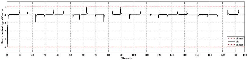
E3S Web of Conferences 229, 01001 (2021) https://doi.org/10.1051/e3sconf/202122901001
ICCSRE’2020
Algorithm 1 CDMPC for RHint control algorithm 64%.
Inputs: Current reference, current state
Output: The optimal control inputs uh or u f
1: Set the systems discrete state space model refer-
ring to 2.3
2: Define and initialize the QP penality matrices and
the MPC prediction horizons for the heater and
fan cases
3: Identify the reference, states and control as sdp
variables
4: Initiaize the reference, the objective and con-
straints
5: for k = 1 : Nh //N f Figure 5: Measured Greenhouse External humidity
6: Solve the optimization problem (8) respecting the
constraints along the prediction horizons Nh or N f In one hand, in Figure 6 and Figure7 and for the
7: endfor
first case, the heater’s behavior under constraints and
8: Extract the first element of the optimal control
the inside’s relative humidity response to the heater
and apply it back to the plant. input control, are presented. It is clearelly shown that
9: end
the heater behaves normally in the presence of con-
straints, hence it attempts his maximum/ minimum
voltage power without exceeding the upper and lower
constraints limits. In Figure 7 the control task was
3 Simulation Results and discusions achieved, here the Humidity decreases from 76% and
tracks smoothly its set point point.
In order to illustrate the (CDMPC) performances,
some numerical simulations were carried out. For
this purpose, we have engaged Model Predictive
Control algorithm using YALMIP Toolbox in MAT-
LAB/Simulink. Using above (QP) algorithm, an op-
timization script function was develloped and the
QUADPROG was choosen as a solver in this case.
For simulation purposes under Simulink an inter-
preted Matlab function block was used for the con-
troller and the plant models representation. To re-
mind, the control objective is to maintain the output
yk of inside humidity RHint, as close as possible to Figure 6: Evolution of the heater Control Signal under Con-
the reference, without exceeding normalized bound- straints
ries 50% ≤ RHint ≤ 75% , besides, the main rea-
son for both identification and control partition, i.e.,
heater and fan cases of study, was based essentially
on how our system works in real life, taking into ac-
count futur real time impplementations.
In order to evaluate the proposed control ap-
proach; for both scenarios, i.e., for the heater and
the fan; the inputs are constrained to evolve between
0 ≤ uh ≤ 5 as voltage applied to the heater and 0 ≤
u f ≤ 4.5 as voltage applied to the fan. The penal-
ity weights were chosen scalars as follows Qh = 100 Figure 7: Hint Response to the heater as Control signal ”uh”
and Rh = 0.1 for the first system and Q f = 100 and
R f = 0.01 for the second one, the prediction horizons In another hand, Figure 8 and Figure 9 show re-
were set to Nh = 40 and N f = 40. As a sample time, spectively, the fan as a second actuator’s behavior, in
Ts was set to 5 seconds. addition to the control task in presence of constraints
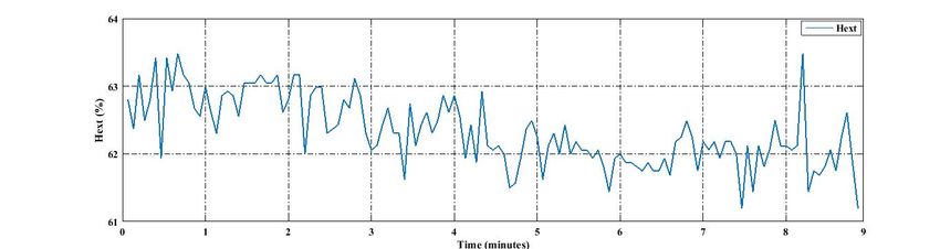
Figure 5 describes the evolution of External rele- for the inside humidity control. It is remarquable
tive humidity for 9 minutes, this evolution shows that that the fan control signal, tends to respect the input
the external humidity varies between a range 61% to constraints and does not exceed 4.5 Volts. However,
5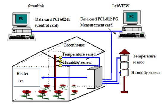
E3S Web of Conferences 229, 01001 (2021)                                                          https://doi.org/10.1051/e3sconf/202122901001
ICCSRE’2020

          several stopping moments are observed, which con-                of inside greenhouse humidity; respecting the con-
          tributes to power saving and actuator durability. Fig-           straints on the controlled inputs condition; have been
          ure 9 presents the control mission, which is eventu-             treated using a (QP) optimization algorithm with nu-
          ally noticed in the internal humidity setpoint tracking,         merical simulations by the means of new optomiza-
          respecting the desired humidity percentage limits. We            tion toolbox as Yalmip.
          can notice that the humidity increases from about                    We have shown that the presented control problem
          59% to attend the setpoint variation range which is              application is solved for the SISO greenhouse system
          64% to 65%.                                                      as a case of study. For a futur task, one of our perspec-
                                                                           tives would be the application and the real time imple-
                                                                           mentation of these approachs for Multi-Input Multi-
                                                                           Output (MIMO) systems and for other climatic pa-
                                                                           rameters control as well.

                                                                           REFERENCES
                                                                           Carrión, I. M., Antúnez, E. A., Castillo, M., and Canals, J.
                                                                                 (2011). A prediction method for nonlinear time se-
                                                                                 ries analysis by combining the false nearest neighbors
                                                                                 and subspace identification methods. Int J Appl Math
          Figure 8: Evolution of the Fan Control Signal under Con-               Inform, 5:258–265.
          straints                                                         Ding, Y., Wang, L., Li, Y., and Li, D. (2018). Model pre-
                                                                                 dictive control and its application in agriculture: A
                                                                                 review. Computers and Electronics in Agriculture,
                                                                                 151:104–117.
                                                                           Eddahhak, A., Lachhab, A., Ezzine, L., and Bouchikhi,
                                                                                 B. (2007). Performance evaluation of a developing
                                                                                 greenhouse climate control with a computer system.
                                                                                 AMSE Journal Modelling C, 68(1):53–64.
                                                                           Faiz, S. E. and Benzaouia, A. (2019). Robust pole place-
                                                                                 ment with minimum gain for constrained linear sys-
                                                                                 tems. In 2019 6th International Conference on Con-
                                                                                 trol, Decision and Information Technologies (CoDIT),
           Figure 9: Hint Response to the Fan as Control signal ”uf”             pages 1127–1131. IEEE.
                                                                           Gandhi, S. V. and Thakker, M. T. (2020). Climate con-
              It is worth noting that, the control method prooves                trol of greenhouse system using neural predictive con-
          a good performance in presence of the constraints on                   troller. In Renewable Energy and Climate Change,
                                                                                 pages 211–221. Springer, file = F.
          the control, despites some damping comportemnt re-
                                                                           Guerbaoui, M., Ed-Dahhak, A., ElAfou, Y., Lachhab, A.,
          garding the control action behavior at the first few
                                                                                 Belkoura, L., and Bouchikhi, B. (2013). Implementa-
          seconds. In general, one might resume that the con-                    tion of direct fuzzy controller in greenhouse based on
          trol task in form of simulation results was succesfully                labview. International journal of electrical and elec-
          granteed.                                                              tronics engineering studies, 1(1):1–13.
              As main futur perspectives, the application and              Hamidane, H., Elfaiz, S., Guerbaoui, M., Ed-dahhak, A.,
          enhancement of the proposed control strategy and its                   Lachhab, A., and Bouchikhi, B. (2020). Pole place-
          real time implementation will be taken in charge, hop-                 ment enhancement of a constrained greenhouse siso
          ing that these initiatives can lead us to novel results.               system. In 2020 1st International Conference on Inno-
                                                                                 vative Research in Applied Science, Engineering and
                                                                                 Technology (IRASET), pages 1–6. IEEE.
                                                                           Lijun, C., Shangfeng, D., Yaofeng, H., and Meihui, L.
          4    Conclusion                                                        (2018). Linear quadratic optimal control applied to
                                                                                 the greenhouse temperature hierarchal system. IFAC-
                                                                                 PapersOnLine, 51(17):712–717.
              In this paper, we have shown a Constrained Dis-
                                                                           Lofberg, J. (2004). Yalmip: A toolbox for modeling and op-
          crete Model Predictive Control (CDMPC) for discrete                    timization in matlab. In 2004 IEEE international con-
          time linear SISO system applicaton for relative hu-                    ference on robotics and automation (IEEE Cat. No.
          midity control. Necessary and sufficient conditions                    04CH37508), pages 284–289. IEEE.
          for the synthesis of the elaborated controller that en-          Mohamed, S. and Hameed, I. (2018). A ga-based adaptive
          sure the desired reference signal tracking and control                 neuro-fuzzy controller for greenhouse climate control

                                                                       6
E3S Web of Conferences 229, 01001 (2021) https://doi.org/10.1051/e3sconf/202122901001
ICCSRE’2020
system. Alexandria Engineering Journal, 57(2):773–
779.
Moufid, A. and Bennis, N. (2019). A multi-modelling ap-
proach and optimal control of greenhouse climate. In
Recent Advances in Electrical and Information Tech-
nologies for Sustainable Development, pages 201–
208. Springer.
Outanoute, M., Lachhab, A., Ed-Dahhak, A., Guerbaoui,
M., Selmani, A., and Bouchikhi, B. (2016). Synthe-
sis of an optimal dynamic regulator based on linear
quadratic gaussian (lqg) for the control of the rela-
tive humidity under experimental greenhouse. Inter-
national Journal of Electrical & Computer Engineer-
ing (2088-8708), 6(5).
Santana, D. D., Martins, M. A., and Odloak, D. (2020).
An efficient cooperative-distributed model predictive
controller with stability and feasibility guarantees for
constrained linear systems. Systems & Control Let-
ters, 141:104701.
Taki, M., Ajabshirchi, Y., Ranjbar, S. F., Rohani, A., and
Matloobi, M. (2016). Heat transfer and mlp neural
network models to predict inside environment vari-
ables and energy lost in a semi-solar greenhouse. En-
ergy and Buildings, 110:314–329.
Wang, F., Mei, X., Rodriguez, J., and Kennel, R. (2017).
Model predictive control for electrical drive systems-
an overview. CES Transactions on Electrical Ma-
chines and Systems, 1(3):219–230.
Wang, Y., Salvador, J. R., de la Pena, D. M., Puig, V., and
Cembrano, G. (2018). Economic model predictive
control based on a periodicity constraint. Journal of
Process Control, 68:226–239.
Xu, X., Sun, Y., Krishnamoorthy, S., and Chandran, K.
(2020). An empirical analysis of green technol-
ogy innovation and ecological efficiency based on a
greenhouse evolutionary ventilation algorithm fuzzy-
model. Sustainability, 12(9):3886.
7You can also read