Branching Processes Modelling for Coronavirus (COVID'19) Pandemic
←
→
Page content transcription
If your browser does not render page correctly, please read the page content below
Branching Processes Modelling for Coronavirus
                      (COVID’19) Pandemic

                               Maroussia Slavtchova-Bojkova 1, 2
     1
         Faculty of Mathematics and Informatics, Sofia University, No5, J. Bourchier Blvd.,
                                        1164 Sofia, Bulgaria
            2
              Institute of Mathematics and Informatics. Bulgarian Academy of Sciences
                                     bojkova@fmi.uni-sofia.bg

         Abstract. The purpose of this paper is to review the recent results in the area of
         infectious disease modelling using general branching processes. A new simulation
         method oriented to model the spread of the COVID’19 pandemic caused by
         SARS-CoV-2 coronavirus is proposed. General branching models turned out to be
         more appropriate and flexible for describing the spread of an infection in a given
         population, than discrete time ones. Concretely, Crump-Mode-Jagers branching
         processes are considered as proper candidates of infectious diseases modelling
         with incubation period like measles, mumps, avian flu, etc. It can be noted that the
         developed methodology is applicable to the diseases that follow the so-called SIR
         (susceptible-infected-removed) and SEIR (susceptible exposed-infected-removed)
         scheme in terms of epidemiological models. Different forecasts are proposed and
         compared on the ground of real data and simulation examples.

         Keywords: SARS-CoV-2 coronavirus, basic reproduction number, general branch-
         ing processes

1   Introduction
Since the Covid-19 pandemic outbreak, a large number of researchers started to
model the pandemic with various mathematical models, and placed their results
on the Internet; see e.g. [1], [2], [3]. However, the number of peer-reviewed
papers is, for now, rather small, especially concerning the branching models used
for this particular kind of pandemic. Hence, another objective of this paper is to
contribute to the discussion on the coronavirus trajectory with the specific kind of
branching processes modelling and for a pandemic caused by a newly emerged
vector-borne disease.
   Branching processes have been applied widely to model epidemic spread (see
for example the monographs by Andersson and Britton [4], Daley and Gani [5]
and Mode and Sleeman [6]. The process describing the number of infectious
individuals in an epidemic model may be well approximated by a branching

 Copyright © 2020 for this paper by
                                 115its authors. Use permitted under
 Creative Commons License Attribution 4.0 International (CC BY 4.0).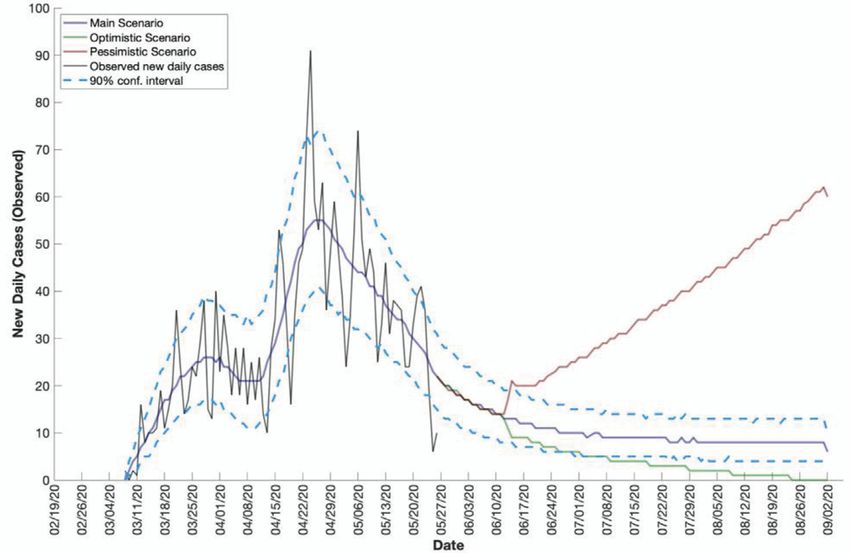
process if the population is homogeneously mixing and the number of infectious
individuals is small in relation to the total size of the susceptible population,
since under these circumstances the probability that an infectious contact is with
a previously infected individual is negligible (see, for example, Isham [7]). Such
an approximation dates back to the pioneering works of Bartlett [8] and Kendall
[9], and can be made mathematically precise by showing convergence of the
epidemic process to a limiting branching process as the number of susceptible
tends to infinity (see Ball [10], Ball and Donnelly [11] and Metz [12]). The
approximation may also be extended to epidemics in populations that are not
homogeneously mixing, for example those containing small mixing units such as
households and workplaces (see Pellis et al. [13]).
   In nowadays situation with COVID’19 pandemic - without existence of
vaccine, the non-pharmaceutical measures, like isolation, quarantine, lock downs,
etc., have been applied all over the world. We are now still in the circumstances of
ongoing pandemic and many typical questions raised are hard to be answered. For
example, what is the basic reproduction number R0 for SARS-CoV-2 coronavirus,
what are the duration outbreak and the size outbreak distributions and others,
concerning the basic quantities needed to be estimated for making forecast.
This work is the first step of incorporating existing knowledge of unknown
characteristics mentioned into the general branching processes (GBP) model. We
are aware of the fact that GBP are specific tool and there are many differences of
COVID’19 disease behavior from one country to another one and moreover from
one particular region in a given country to another one, but the main idea behind
this approach is to treat data available for each country in a unified way, based on
the estimates existing in the scientific literature at the moment for SARS-CoV-2
coronavirus spreading.
   The paper is organized as follows: Section 2 briefly introduces the general
branching processes model, while Section 3 is devoted to the statistical methodology
developed and simulation results. First, the impact of basic reproduction number
R0, reflecting an effect of preventive measures applied on the future behavior
of the epidemics is studied. Second, we apply the methodology for the data set
collected on a daily base and published at Worldometer (see [14]) for Bulgaria,
Belgium and South Korea. For every country, we made 1000 simulations to obtain
the forecast of new cases emergence in three possible scenarios: main, optimistic
and pessimistic. We end up the paper by discussion of the results in Section 4.

2   General Branching Processes Model
Before proceeding we give outline descriptions of some common branching
process models (see e.g. Jagers [15] for further details), which describe the
evolution of a single-type population, which in what follows will be supposed to be

                                        116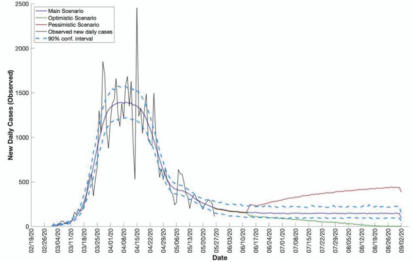
the one of infected individuals. In all of these branching models, individuals have
independent and identically distributed reproduction processes. The reproduction
process in terms of epidemic spread meaning the random process signifying the
new infected by each contact with infectious one. In the case of SARS-CoV-2
coronavirus it is known that each contact results in new infective. If not, this
situation could be incorporated into the model with introducing in addition the
probability that after a contact an individual may not get infection, say with
probability p. In a Bienayme-Galton-Watson branching process, each individual
live for one unit of time and then has a random number of children, distributed
according to a random variable, ξ say. In a Bellman-Harris branching process,
each individual live until a random age, distributed according to a random variable
I say, and then has a random number of children, distributed according to ξ, where
I and ξ are independent. The Sevastyanov branching process is defined similarly,
except I and ξ may be dependent, so the number of children an individual has is
correlated with that individual’s lifetime. In all of the mentioned above classes
of BP there is one feature in common which is distinguishing them as a whole
from the general BP. That is the assumption that every individual after living
a random (or unit) time, dies leaving a random number of ancestries. Finally,
in a general branching process, also called a Crump-Mode-Jagers branching
process (CMJBP), each individual live until a random age, distributed according
to I, and reproduces at ages according to a point process ζ. More precisely, if an
individual, i say having reproduction profile (Ii,ξi), is born at time bi and 0 ≤ τi1
≤ τi2 ≤ ... ≤ Ii denote the points of ξi, then individual i has one child at each of
times bi + τi1, bi + τi2,.... This model permit that a mother could have more than
one child during her life or in terms of epidemic that every contaminated case
could contact and pass the viral infection to more than one susceptible during its
infectious period. However, the situation with SARS-CoV-2 coronavirus is rather
different in comparison to other viruses existed until now. It was reported that
an individual could just transfer the virus without being ill and/or symptomatic,
which complicates the contact process as a whole and the tracing the contacts
consequently.
   This paper is primarily concerned with models for epidemics of diseases,
such as measles, mumps and avian influenza, which follow the so-called SIR
(Susceptible → Infective → Removed) scheme in a closed, homogeneously
mixing population or some of its extensions. A key epidemiological parameter for
such an epidemic model is the basic reproduction number R0 (see Heesterbeek
and Dietz [16]), which in the present setting is given by the mean of the offspring
distribution of the approximating branching process. In particular a major
outbreak (i.e. one whose size is of the same order as the population size) occurs
with non-zero probability if and only if R0 > 1.
   Suppose that R0 > 1 and some preventive transmission measures are taken

                                        117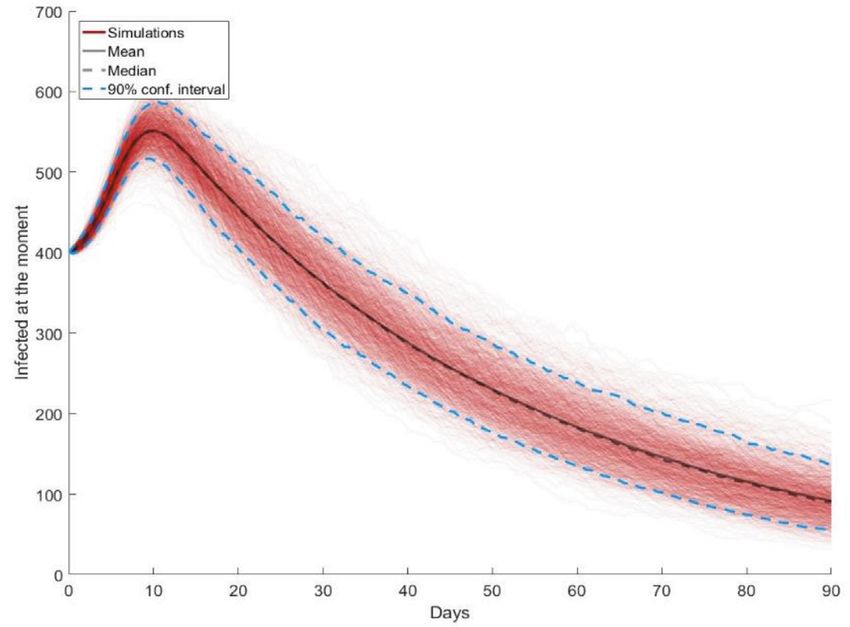
in advance of an epidemic. If there were a vaccine this could be expressed in
such a way that fraction c of the population is vaccinated with a perfect vaccine
in advance of an epidemic. Then R0 is reduced to (1 − c) R0, since a proportion
c of infectious contacts is with vaccinated individuals. It follows that a major
outbreak is almost surely prevented if and only if R0– . This well-known result,
which gives the critical vaccination coverage to prevent a major outbreak and
goes back at least to 1964 (e.g. Smith [17]), is widely used to inform public health
authorities, but if there is a vaccine.
   As a consequence of the above result, many analyses in the epidemic
modelling literature have focussed on reducing R0 to its critical value of one. In
the case of COVID’19 pandemic it is done by closing public institutions, schools,
universities, etc., social isolation, lock downs of towns and/or regions and our
aim is to present an approach of measuring an effect of these measures.

3   Statistical Method and Simulation Results

3.1 The impact of basic reproduction number R0, reflecting an effect of
preventive measures applied
Our methodology is based primarily on the CMJBP as a model of epidemic spread.
It this section by use of the statistical software especially developed for branching
processes simulations [18] we first fit the parameters of the model to the data
available for particular country, as it is obvious that there is a variety of different
behaviours among them. We are interested in the similarities and differences
between them and the reasons they stemmed from. The two main characteristics
running the behaviour of the CMJBP are the distribution of the fertility period
duration of individuals and the point process governing the reproduction process
of any individual, which may depend on the age of individual. These quantities in
terms of epidemic spreading mean the distribution of the serial interval, which is
the sum of incubation period and delay period (see Fig. 1) and the point process
signifying the number of new infected individuals any infective individual, may
pass the virus to.
     Each potential new infection was assigned a time of infection drawn from
the serial interval distribution. Secondary cases were only created if the infector
had not been isolated by the time of infection. In the example in Fig. 1, person
A can potentially produce three secondary infections, but only two transmissions
occur before the case was isolated. Thus, a reduced delay from onset to isolation
reduces the average number of secondary cases in the model.
     It is important to say that the notion of “age” in the epidemic context means

                                         118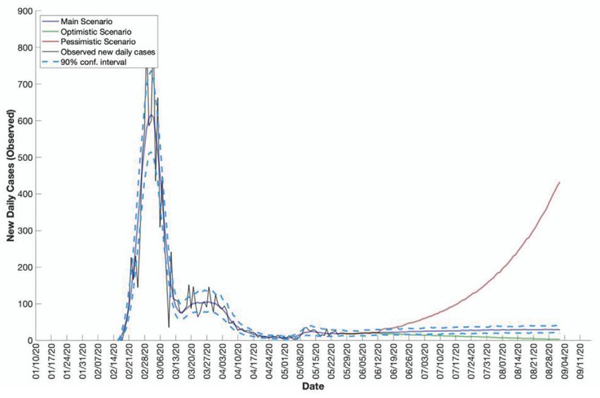
the “stage” of the disease in the human organism and consequently the number
of newly infected individuals emerging from the contact with an infectious one
is depending on the phase at which the infected individual passes the disease.
That is why we model the serial interval (see [19]) as a sum of incubation period
during which an infected individual is asymptomatic but could transmit the virus
and a delay period which is the interval after the symptoms appeared (and the
infected individual may pass the virus to the contacted one or may not if he or she
is being isolated) up to the time of isolation.
In the present study for the parameters of the general branching process, we
use the left-truncated normal distribution N(35,5.12), using known estimates from
[19] that the incubation period is distributed by an average of 5.8 and a standard
deviation of 2.6 and in the absence of any measures, the contagious individual is
not isolated, i.e. he or she infects other people throughout the infection. However,
if there is an isolation of the infected case after symptoms have emerged,
to incorporate this event into the model, we should take this into account by
introducing another distribution of delay time between the onset of symptoms
and the isolation, which is judged to be with mean 3.83 and dispersion 5.99 (see
[19]). For the point process modelling the number of infected individuals by one
infected, we use gamma distribution with appropriately defined parameters, i.e.
Γ (7.2734,1.3240) (see [19]).
There are many estimates of the reproduction number for the early phase
of the SARS-CoV-2 outbreak in Wuhan, China (see [19] and the references
therein) and therefore we used the values 1.5, 2.5, and 3.5, which span most of
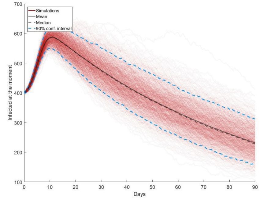
the range of current estimates. For any particular value of R0 = 1;1.5;2.5, 1000
simulations have been made using the statistical software especially developed
for branching processes simulations [18], which reveal the behaviour of the
number of contaminated at a given time by taking additional measures to isolate,
quarantine and block certain areas. The effect of the measures taken in reducing
this number is seen as an estimate of the number of infected individuals in Fig.
2 and 3, while in the absence of such measures as in Fig. 4 and 5 this number
is increasing. In both cases, however, for the selected parameters of the general
branching process, the horizon of 90 days from the onset of the infection in the
population is short to can claim that the epidemic is eliminated within this period.
119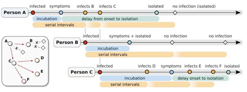
Fig. 1. An example of serial interval

Fig. 2. Forecast of new cases at certain time under mitigation interventions, when R0 = 1, i.e. the
                                   branching process is critical

                                               120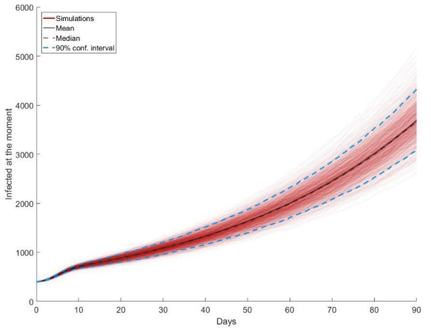
Fig. 3. Forecast of new cases at certain time under mitigation interventions, when R0 = 1.093, i.e.
                         the branching process is slightly super-critical

Fig. 4. Forecast of new cases at certain time without mitigation interventions, when R0 = 1.5, i.e.
                              the branching process is supercritical

                                               121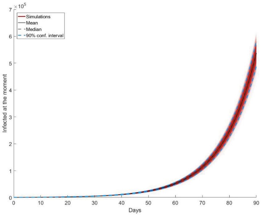
Fig. 5. Forecast of new cases at certain time without mitigation interventions, when R0 = 1.5, i.e.
                              the branching process is supercritical

3.2 Forecasts of COVID’19 development in Bulgaria
In this subsection, we are illustrating the methodology using the CMJBP after
fitting the theoretical model to the historical data published at Worldometer (see
[14]). This way we acquire the values, which are best revealing and explaining
the structure of the historical data representing the new daily cases and total
cases, as well. Then with the values of estimated parameters - R0 and the serial
interval distribution, giving the best fit to the data, we are projecting further the
behaviour of the new daily cases in three scenarios. The main scenario is when
for the forecast we used the estimated value of R0, for the optimistic scenario we
decrease the estimated value of R0 and for the pessimistic one - we increase R0.
On Fig. 6, one can see the results of the fit of the model (in blue) vs observed (in
black) total cases and on Fig. 7 of the fit of the model (in blue) vs observed (in
black) new daily cases, both for Bulgaria. On Fig. 8 are presented the forecasts
for Bulgaria by three scenarios: main (in lilac) together with the 90% confidence
interval, optimistic (in green), pessimistic (in brown) and the actual new daily
cases (in black) using the data from the beginning of the infection on March 8,
2020 up to May 27, 2020. So following the graphics on Fig. 8 one can see in the
period after May 27, 2020 up to approximately June 10, 2020 the fit between the

                                               122
model vs observed new daily cases is very good, but after that it is possible to
have three possible trajectories according to the three different scenarios all of
them projecting to September 2, 2020.
Fig. 6. The comparison between the model vs observed total cases for Bulgaria
123Fig. 7. The comparison between the model vs observed new daily cases for Bulgaria
Fig. 8. Forecast of new daily cases in Bulgaria by three scenarios: main, optimistic and
pessimistic ones using the data from Worldometer
1243.3 Forecasts of COVID’19 development in Belgium
The results for Belgium are presented on Fig. 9, where is the fit of the model (in
blue) vs observed (in black) total cases and on Fig. 10 is the fit of the model (in
blue) vs observed (in black) new daily cases. Then, on Fig. 11 one could see the
forecasts for Belgium by three scenarios: main (in lilac) together with the 90%
confidence interval, optimistic (in green), pessimistic (in brown) for the actual
new daily cases (in black) using the data from the beginning of the infection on
March 8, 2020 up to May 27, 2020. It is interesting to note that the epidemic started
at the same time in Bulgaria and Belgium and that is one of the reasons to choose
to present here the results for these two countries. So following the graphics on
Fig. 11 one can see in the period after May 27, 2020 up to approximately June
10, 2020 the fit between the model vs observed new daily cases is very good, but
after that it is possible to have three possible trajectories according to the three
different scenarios all of them projecting to September 2, 2020. Also, as it could
be seen the behaviour by pessimistic scenario in Belgium is rather different from
that in Bulgaria and one of the reasons for that is the difference in the outbreak
smoothing curve corresponding to new daily cases in Bulgaria (see Fig. 8) and
that for Belgium (see Fig. 11).
Fig. 9. The comparison between the model vs observed total cases for Belgium
125Fig. 10. The comparison between the model vs observed new daily cases for Belgium
Fig. 11. Forecast of new daily cases in Belgium by three scenarios: main, optimistic and
pessimistic ones using the data from Worldometer
1263.4 Forecasts of COVID’19 development in South Korea
The case of South Korea turned out to be quite different from those of Bulgaria and
Belgium. It is known that in South Korea, the measures applied are technological
and this country does not take social isolation and other typical measures we
already mentioned before. Rather, the tracing of contacts together with the
secondary cases is taken with high probability.
First, one can see the difference in the results of the fit of the model vs observed
total cases between South Korea (Fig. 12) and those for Bulgaria (see Fig. 6) and
Belgium (see Fig. 9). The curves of total cases for South Korea (Fig. 12) are
steeper than those for Bulgaria (see Fig. 6) and Belgium (see Fig. 9) which has its
explanation in the different policies followed in the three countries.
Second, because of measures taken in South Korea on Fig. 13, one could
observe that the smoothing model curve for daily outbreaks has different behaviour
in comparison to those of Bulgaria and Belgium. It is because the limitations are
not so strict in South Korea, which is resulting in a faster growth, than in the other
two countries, of the size of new daily cases and the appearance of the second wave.
Because of that scenario accepted in South Korea, however, there is a possibility of
the next major outbreak in that country, as it is presented on Fig. 14.
Fig. 12. The comparison between the model vs observed total cases for South Korea
127Fig. 13. The comparison between the model vs observed new daily cases for South Korea
Fig. 14. Forecast of new daily cases in South Korea by three scenarios: main, optimistic and
pessimistic ones using the data from Worldometer
1284 Discussion
In this paper, we have presented a mathematical tool to tackle infectious disease
outbreaks in order to estimate the impact of preventive measures applied. In
particular, this tool addresses various technical questions posed by the author to
support the ongoing public health response to COVID-19. This approach considers
both estimation efforts for key parameters, and investigative efforts (often-
numerical simulations) in assessing the effectiveness of various intervention or
control measures. Mutual concern of estimation and simulation efforts is critical.
Parameter estimates are obtained using a certain set of assumptions regarding the
data, and investigations or simulations utilising these estimates should guarantee
that their underlying assumptions are consistent. These challenges in model
construction and applicability of statistical methods become more complex by
the limitations of the data with which decisions must be made.
There are many complications when modelling an outbreak of a novel
infectious disease. To address some of these, we have described a possible
technique to serve as part of a generally applicable toolkit. However, our proposed
model, and many other models, are subject to important restrictions, which must
be considered prior to their application. Significant among these are the lack
of heterogeneous population mixing, such as through age and different risk-
groups, and spatio-temporal variations all of which have an impact on modelling
estimates and predictions.
Nevertheless, the relative simplicity of the presented model allows for the
development of qualitative intuition regarding the efficacy of various intervention
methods, whilst providing tractable theoretical frameworks, which can be further,
developed and better inform policy-makers.
5 Acknowledgements
This work was supported by the project BG05M2OP001-1.001-0004 (UNITe)
funded by Operational Program Science and Education for Smart Growth co-
funded by European Regional Development Fund for theoretical development
of the stochastic modelling of COVID’19 pandemic by means of branching
processes and for computational resources by the project KP-6-H22/3 of NSF at
the Bulgarian Ministry of Education and Science.
The author also would like to express her gratitude to her colleagues Plamen
Trayanov and Valeriya Simeonova for their continuous support on the computer
implementations and to the anonymous referees for their careful reading of the
manuscript and useful comments and suggestions, which improved the quality of
the paper.
129References
1. W.W. Koczkodaj, M.A. Mansournia, W. Pedrycz, A.Wolny-Dominiak, P.F. Zabrodskii, D. Str-
zalka, T. Armstrong, A.H. Zolfaghari, M. Debski, J. Mazurek: 1,000,000 cases of COVID-19
outside of China: The date predicted by a simple heuristic, Global Epidemiology, (2020)
2. Lixiang Li and Zihang Yang, Zhongkai Dang, Cui Meng, Jingze Huang, Haotian Meng, Deyu
Wang, Guanhua Chen, Jiaxuan Zhang, Haipeng Peng, Yiming Shao: Propagation analysis and
prediction of the COVID-19, Infectious Disease Modelling, 5, 282–292. (2020)
3. Petropoulos, F., Makridakis, S.: Forecasting the novel coronavirus COVID19, PLoS ONE,
https://doi.org/10.1371/journal.pone.0231236 (2000).
4. Andersson, H. and Britton, T.: Stochastic Epidemic Models and Their Statistical Analysis.
Lecture Notes in Statistics, 151. New York: Springer. (2000)
5. Daley, D.J., Gani, J.: Epidemic Modelling: An Introduction. Cambridge Studies in Mathemati-
cal Biology 15. Cambridge: Cambridge Univ. Press. (1999)
6. Mode, C.J., Sleeman, C.K.: Stochastic Processes in Epidemiology. Singapore: World Scien-
tific. (2000)
7. Isham, V.: Stochastic models for epidemics. In Celebrating Statistics. Oxford Statist. Sci. Ser.
33 (A.C. Davison, Y. Dodge and N. Wermuth, eds.) 27–54. Oxford: Oxford Univ. Press. (2005)
8. Bartlett, M.S.: An Introduction to Stochastic Processes, 1st ed. Cambridge: Cambridge Univ.
Press. (1955)
9. Kendall, D.G.: Deterministic and stochastic epidemics in closed populations. In Proceedings
of the Third Berkeley Symposium on Mathematical Statistics and Probability, IV, 149–165.
Berkeley and Los Angeles: Univ. California Press. (1956)
10. Ball, F.: The threshold behaviour of epidemic models. J. Appl. Probab. 20, 227–241. (1983)
11. Ball, F., Donnelly, P.: Strong approximations for epidemic models. Stochastic Process. Appl.,
55, 1–21. (1995)
12. Metz, J.: The epidemic in a closed population with all susceptibles equally vulnerable; some
results for large susceptible populations and small initial infections. Acta Biotheoretica, 27,
75–123, (1978)
13. Pellis, L., Ball, F., Trapman, P.: Reproduction numbers for epidemic models with households
and other social structures. I. Definition and calculation of R0. Math. Biosci., 235, 85–97.
(2012)
14. https://www.worldometers.info/coronavirus/countries
15. Jagers, P.: Branching Processes with Biological Applications. London: Wiley. (1975)
16. Heesterbeek, J.A.P., Dietz, K.: The concept of R0 in epidemic theory. Statist. Neerlandica, 50,
89–110. (1996)
17. Smith, C.E.G.: Factors in the transmission of virus infections from animal to man. Scientific
Basis of Medicine Annual Review, 125–150. London: Athlone Press. (1964)
18. Plamen Trayanov. Branching Process Simulator (https://www.github.com/plamentrayanov/
BranchingProcessSimulator), GitHub. (2018)
19. Hellewell J., Abbott S. , Gimma A., et all: Feasibility of controlling 2019-nCoV outbreaks by
isolation of cases and contacts. https://doi.org/10.1101/2020.02.08.20021162 (2020)
130You can also read