InteractiveDisplay: A package for enabling interactive visualization of Bioconductor objects - Shawn Balcome March 8, 2021
←
→
Page content transcription
If your browser does not render page correctly, please read the page content below
interactiveDisplay: A package for enabling interactive
         visualization of Bioconductor objects
                      Shawn Balcome
                      March 8, 2021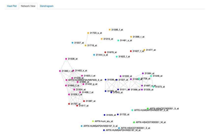
interactiveDisplay: A package for enabling interactive visualization of Bioconductor objects                                                                                                   1

Contents
List of Figures                                                                                                                                                                                1

1 Introduction                                                                                                                                                                                 2

2 Installation                                                                                                                                                                                 2

3 Support                                                                                                                                                                                      3

4 Citation                                                                                                                                                                                     3

5 Bioconductor Object Methods                                                                                                                                                                  3
  5.1 GRanges and GRangesList . . . . . . . .         .   .   .   .   .   .   .   .   .   .   .   .   .   .   .   .   .   .   .   .   .   .   .   .   .   .   .   .   .   .   .   .   .   .    4
      5.1.1 Object Background - GRanges . .           .   .   .   .   .   .   .   .   .   .   .   .   .   .   .   .   .   .   .   .   .   .   .   .   .   .   .   .   .   .   .   .   .   .    4
      5.1.2 Object Background - GRangesList           .   .   .   .   .   .   .   .   .   .   .   .   .   .   .   .   .   .   .   .   .   .   .   .   .   .   .   .   .   .   .   .   .   .    5
      5.1.3 Method . . . . . . . . . . . . . .        .   .   .   .   .   .   .   .   .   .   .   .   .   .   .   .   .   .   .   .   .   .   .   .   .   .   .   .   .   .   .   .   .   .    6
      5.1.4 UI . . . . . . . . . . . . . . . . .      .   .   .   .   .   .   .   .   .   .   .   .   .   .   .   .   .   .   .   .   .   .   .   .   .   .   .   .   .   .   .   .   .   .    6
      5.1.5 Plots . . . . . . . . . . . . . . . .     .   .   .   .   .   .   .   .   .   .   .   .   .   .   .   .   .   .   .   .   .   .   .   .   .   .   .   .   .   .   .   .   .   .    8
      5.1.6 Metadata Tabset . . . . . . . . .         .   .   .   .   .   .   .   .   .   .   .   .   .   .   .   .   .   .   .   .   .   .   .   .   .   .   .   .   .   .   .   .   .   .   10
  5.2 ExpressionSet . . . . . . . . . . . . . . .     .   .   .   .   .   .   .   .   .   .   .   .   .   .   .   .   .   .   .   .   .   .   .   .   .   .   .   .   .   .   .   .   .   .   10
      5.2.1 Object Background . . . . . . . .         .   .   .   .   .   .   .   .   .   .   .   .   .   .   .   .   .   .   .   .   .   .   .   .   .   .   .   .   .   .   .   .   .   .   10
      5.2.2 Method . . . . . . . . . . . . . .        .   .   .   .   .   .   .   .   .   .   .   .   .   .   .   .   .   .   .   .   .   .   .   .   .   .   .   .   .   .   .   .   .   .   11
      5.2.3 UI . . . . . . . . . . . . . . . . .      .   .   .   .   .   .   .   .   .   .   .   .   .   .   .   .   .   .   .   .   .   .   .   .   .   .   .   .   .   .   .   .   .   .   11
      5.2.4 Plots . . . . . . . . . . . . . . . .     .   .   .   .   .   .   .   .   .   .   .   .   .   .   .   .   .   .   .   .   .   .   .   .   .   .   .   .   .   .   .   .   .   .   14
      5.2.5 GO Tabset . . . . . . . . . . . . .       .   .   .   .   .   .   .   .   .   .   .   .   .   .   .   .   .   .   .   .   .   .   .   .   .   .   .   .   .   .   .   .   .   .   16
  5.3 RangedSummarizedExperiment . . . . . .          .   .   .   .   .   .   .   .   .   .   .   .   .   .   .   .   .   .   .   .   .   .   .   .   .   .   .   .   .   .   .   .   .   .   18
      5.3.1 Object Background . . . . . . . .         .   .   .   .   .   .   .   .   .   .   .   .   .   .   .   .   .   .   .   .   .   .   .   .   .   .   .   .   .   .   .   .   .   .   18
      5.3.2 Method . . . . . . . . . . . . . .        .   .   .   .   .   .   .   .   .   .   .   .   .   .   .   .   .   .   .   .   .   .   .   .   .   .   .   .   .   .   .   .   .   .   19
      5.3.3 UI . . . . . . . . . . . . . . . . .      .   .   .   .   .   .   .   .   .   .   .   .   .   .   .   .   .   .   .   .   .   .   .   .   .   .   .   .   .   .   .   .   .   .   19
      5.3.4 Plot . . . . . . . . . . . . . . . .      .   .   .   .   .   .   .   .   .   .   .   .   .   .   .   .   .   .   .   .   .   .   .   .   .   .   .   .   .   .   .   .   .   .   19

6 Additional Functions/Methods                                                                                                                                                                19
  6.1 Dataframe - display() . . . . . . . . . . . . . . . . . . . . . . . . . . . . . . . . . . . . . . . . . . . . .                                                                         19
  6.2 Dataframe - simplenet() . . . . . . . . . . . . . . . . . . . . . . . . . . . . . . . . . . . . . . . . . . . .                                                                         20
  6.3 gridsvgjs() . . . . . . . . . . . . . . . . . . . . . . . . . . . . . . . . . . . . . . . . . . . . . . . . . . .                                                                       21

7 Special Mention Components                                                                                                                                                                  21
  7.1 Shiny . . . . . . . . . . . . . . . . . . . . . . . . . . . . . . . . . . . . . . . . . . . . . . . . . . . . . .                                                                       21
  7.2 Gviz/ggbio . . . . . . . . . . . . . . . . . . . . . . . . . . . . . . . . . . . . . . . . . . . . . . . . . . .                                                                        21
  7.3 gridSVG . . . . . . . . . . . . . . . . . . . . . . . . . . . . . . . . . . . . . . . . . . . . . . . . . . . .                                                                         21

8 JavaScript Libraries                                                                                                                                                                        22
  8.1 Data-Driven Documents . . . . . . . . . . . . . . . . . . . . . . . . . . . . . . . . . . . . . . . . . . . .                                                                           22
  8.2 Zoom/Pan JavaScript libraries . . . . . . . . . . . . . . . . . . . . . . . . . . . . . . . . . . . . . . . .                                                                           22
  8.3 JavaScript Color Chooser . . . . . . . . . . . . . . . . . . . . . . . . . . . . . . . . . . . . . . . . . . .                                                                          22

9 Acknowledgments                                                                                                                                                                             22

10 SessionInfo                                                                                                                                                                                23

11 References                                                                                                                                                                                 24

List of Figures
   1     GRange, Chromosome drop-down menus . . . . . . . . . . . . . . . . . . . . . . . . . . . . . . . . . . .                                                                              6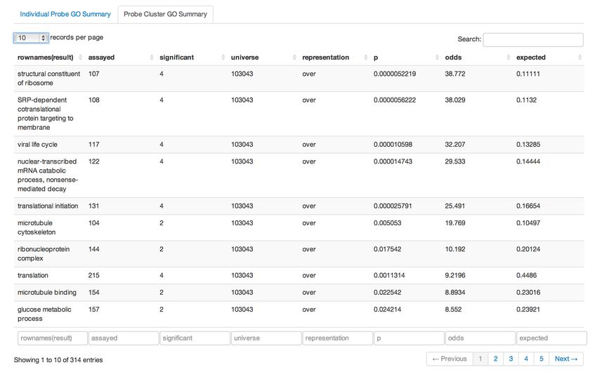
interactiveDisplay: A package for enabling interactive visualization of Bioconductor objects                                                              2

    2    UCSC Genome drop-down, Suppress Ideogram checkbox . . . . . . . . . . . .               .   .   .   .   .   .   .   .   .   .   .   .   .   .    7
    3    Plot Window Range slider, Length Filter slider, Choose a Strand drop-down . .           .   .   .   .   .   .   .   .   .   .   .   .   .   .    7
    4    Deposit Ranges in View button, Clear Deposit button, Save to Console button             .   .   .   .   .   .   .   .   .   .   .   .   .   .    7
    5    Static Circle Layout . . . . . . . . . . . . . . . . . . . . . . . . . . . . . . . .    .   .   .   .   .   .   .   .   .   .   .   .   .   .    8
    6    Interactive Plot . . . . . . . . . . . . . . . . . . . . . . . . . . . . . . . . . .    .   .   .   .   .   .   .   .   .   .   .   .   .   .    8
    7    All Ranges in Object . . . . . . . . . . . . . . . . . . . . . . . . . . . . . . . .    .   .   .   .   .   .   .   .   .   .   .   .   .   .    9
    8    Selected Ranges in Current View . . . . . . . . . . . . . . . . . . . . . . . . .       .   .   .   .   .   .   .   .   .   .   .   .   .   .    9
    9    Deposited Selections . . . . . . . . . . . . . . . . . . . . . . . . . . . . . . . .    .   .   .   .   .   .   .   .   .   .   .   .   .   .    9
    10   Dynamically Created Metadata Tabs . . . . . . . . . . . . . . . . . . . . . . .         .   .   .   .   .   .   .   .   .   .   .   .   .   .   10
    11   Experiment Info . . . . . . . . . . . . . . . . . . . . . . . . . . . . . . . . . .     .   .   .   .   .   .   .   .   .   .   .   .   .   .   11
    12   Suppress Heatmap checkbox, Transpose Heatmap checkbox . . . . . . . . . . .             .   .   .   .   .   .   .   .   .   .   .   .   .   .   11
    13   Network/Dendrogram View dropdown . . . . . . . . . . . . . . . . . . . . . .            .   .   .   .   .   .   .   .   .   .   .   .   .   .   12
    14   Group Wide GO Summary UI . . . . . . . . . . . . . . . . . . . . . . . . . . .          .   .   .   .   .   .   .   .   .   .   .   .   .   .   12
    15   Individual Probe GO Summary dropdown . . . . . . . . . . . . . . . . . . . .            .   .   .   .   .   .   .   .   .   .   .   .   .   .   12
    16   Subset UI . . . . . . . . . . . . . . . . . . . . . . . . . . . . . . . . . . . . .     .   .   .   .   .   .   .   .   .   .   .   .   .   .   12
    17   Tweak Axis Label Font Size slider . . . . . . . . . . . . . . . . . . . . . . . .       .   .   .   .   .   .   .   .   .   .   .   .   .   .   13
    18   Edge/Distance UI . . . . . . . . . . . . . . . . . . . . . . . . . . . . . . . . .      .   .   .   .   .   .   .   .   .   .   .   .   .   .   13
    19   Force Layout sliders . . . . . . . . . . . . . . . . . . . . . . . . . . . . . . . .    .   .   .   .   .   .   .   .   .   .   .   .   .   .   13
    20   Clustering UI . . . . . . . . . . . . . . . . . . . . . . . . . . . . . . . . . . . .   .   .   .   .   .   .   .   .   .   .   .   .   .   .   13
    21   Color Picker UI . . . . . . . . . . . . . . . . . . . . . . . . . . . . . . . . . .     .   .   .   .   .   .   .   .   .   .   .   .   .   .   14
    22   Stop Application button . . . . . . . . . . . . . . . . . . . . . . . . . . . . . .     .   .   .   .   .   .   .   .   .   .   .   .   .   .   14
    23   Heat Plot . . . . . . . . . . . . . . . . . . . . . . . . . . . . . . . . . . . . .     .   .   .   .   .   .   .   .   .   .   .   .   .   .   14
    24   Network View - Samples . . . . . . . . . . . . . . . . . . . . . . . . . . . . .        .   .   .   .   .   .   .   .   .   .   .   .   .   .   15
    25   Network View - Probes . . . . . . . . . . . . . . . . . . . . . . . . . . . . . .       .   .   .   .   .   .   .   .   .   .   .   .   .   .   15
    26   Dendrogram - Samples . . . . . . . . . . . . . . . . . . . . . . . . . . . . . .        .   .   .   .   .   .   .   .   .   .   .   .   .   .   16
    27   Dendrogram - Probes . . . . . . . . . . . . . . . . . . . . . . . . . . . . . . .       .   .   .   .   .   .   .   .   .   .   .   .   .   .   16
    28   Individual Probe GO Summary . . . . . . . . . . . . . . . . . . . . . . . . . .         .   .   .   .   .   .   .   .   .   .   .   .   .   .   17
    29   Probe Cluster GO Summary . . . . . . . . . . . . . . . . . . . . . . . . . . . .        .   .   .   .   .   .   .   .   .   .   .   .   .   .   17
    30   RangedSummarizedExperiment UI . . . . . . . . . . . . . . . . . . . . . . . .           .   .   .   .   .   .   .   .   .   .   .   .   .   .   19
    31   Binned Mean Counts by Position . . . . . . . . . . . . . . . . . . . . . . . . .        .   .   .   .   .   .   .   .   .   .   .   .   .   .   19
    32   Dataframe Table . . . . . . . . . . . . . . . . . . . . . . . . . . . . . . . . . .     .   .   .   .   .   .   .   .   .   .   .   .   .   .   20
    33   simplenet . . . . . . . . . . . . . . . . . . . . . . . . . . . . . . . . . . . . . .   .   .   .   .   .   .   .   .   .   .   .   .   .   .   20
    34   gridSVG [5] . . . . . . . . . . . . . . . . . . . . . . . . . . . . . . . . . . . .     .   .   .   .   .   .   .   .   .   .   .   .   .   .   22

1    Introduction
interactiveDisplay makes use of Bioconductor visualization packages, the Shiny [8] web framework, the D3.js visualization
JavaScript library, and other libraries to produce various web applications built around Bioconductor objects.
Four popular Bioconductor data objects are currently supported: GRanges, GRangesList, ExpressionSet and RangedSum-
marizedExperiment. In addition, the second April 2014 release version now includes a method for data frames and is
imported by the AnnotationHub [1] package.
This vignette will provide some background and guidance on the use of the current supported methods.

2    Installation
The webpage for the release version of interactiveDisplay is available at:
http://bioconductor.org/packages/release/bioc/html/interactiveDisplay.html
And the development version is available at:
http://bioconductor.org/packages/devel/bioc/html/interactiveDisplay.html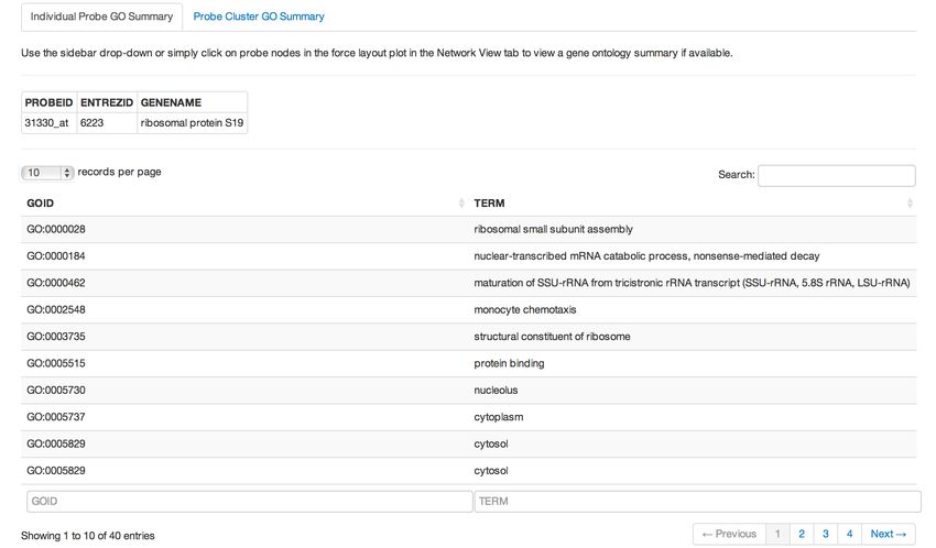
interactiveDisplay: A package for enabling interactive visualization of Bioconductor objects 3
It can also be installed within the R console using BiocManager::install().
if (!requireNamespace("BiocManager", quietly=TRUE))
install.packages("BiocManager")
BiocManager::install("interactiveDisplay")
interactiveDisplay is actively maintained and it may be desirable to use the developer branch of the package. If the user
is willing to install development versions of Bioconductor packages, this can be accomplished by toggling the setting and
reinstalling packages with BiocManager::install(version = ”devel”). The development branch is actively changed, so users
should expect to encounter errors. Generally, development and release versions of packages should not be mixed.
if (!requireNamespace("BiocManager", quietly=TRUE))
install.packages("BiocManager")
BiocManager::install(version = "devel")
BiocManager::install("interactiveDisplay")
Because interactiveDisplay depends on many different R packages, some of which are used in only one individual method,
many dependencies are suggested and will only be required when a method is run for the first time. This helps with load
time when other packages (currently AnnotationHub) import methods from interactiveDisplay. If a required package is
missing when a method is run, a message with instructions on obtaining it will be output in the R console.
3 Support
Send me an email directly at balc0022@umn.edu
Search, subscribe or contact the bioconductor or bioc-devel mailing lists at http://www.bioconductor.org/
help/mailing-list/
4 Citation
citation("interactiveDisplay")
##
## To cite package 'interactiveDisplay' in publications use:
##
## Shawn Balcome and Marc Carlson (2021). interactiveDisplay: Package
## for enabling powerful shiny web displays of Bioconductor objects. R
## package version 1.29.1.
##
## A BibTeX entry for LaTeX users is
##
## @Manual{,
## title = {interactiveDisplay: Package for enabling powerful shiny web displays of Bioconductor
## objects},
## author = {Shawn Balcome and Marc Carlson},
## year = {2021},
## note = {R package version 1.29.1},
## }
##
## ATTENTION: This citation information has been auto-generated from the
## package DESCRIPTION file and may need manual editing, see
## 'help("citation")'.
5 Bioconductor Object Methods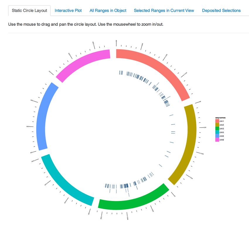
interactiveDisplay: A package for enabling interactive visualization of Bioconductor objects                            4

5.1     GRanges and GRangesList
5.1.1   Object Background - GRanges
The GRanges object is a standardized container for genomic location data used in many Bioconductor packages. It is
built on S4 classes from the the infrastructure package IRanges.
First, load the libraries needed for the examples in this document and load the example GRanges data provided with the
interactiveDisplay package.
options(width=80)
options(continue=" ")
suppressMessages(library(ggplot2))
suppressMessages(library(interactiveDisplay))
suppressMessages(library(Biobase))

data(mmgr)
mmgr
## Loading required package:          GenomicRanges
## Loading required package:          stats4
## Loading required package:          S4Vectors
##
## Attaching package:        ’S4Vectors’
## The following objects are masked from ’package:base’:
##
##    I, expand.grid, unname
## Loading required package:          IRanges
## Loading required package:          GenomeInfoDb
## GRanges object with 1000 ranges and 2 metadata columns:
##          seqnames              ranges strand |       tx_id                             tx_name
##                          |
##      [1]     chr5   53267178-53278539      + |       27296                  ENSMUST00000147148
##      [2]     chr2 170346991-170427845      - |       40171                  ENSMUST00000172093
##      [3]     chr7     4472475-4474584      + |       28623                  ENSMUST00000084338
##      [4]     chr9 123772185-123790939      - |       37251                  ENSMUST00000109152
##      [5]     chr7 127588698-127603605      + |       28623                  ENSMUST00000038824
##      ...      ...                 ...    ... .         ...                                 ...
##    [996]     chr5 129715558-129718290      + |       24633                  ENSMUST00000148260
##    [997]     chr4 115915120-115939926      - |       27296                  ENSMUST00000147148
##    [998]     chr4 116598492-116599164      + |       27296                  ENSMUST00000148260
##    [999]     chr5 124552958-124560784      + |       37251                  ENSMUST00000038824
##   [1000]     chr2 170482708-170497145      - |       40171                  ENSMUST00000172093
##   -------
##   seqinfo: 9 sequences from an unspecified genome

Each row in the GRanges object represents an individual range using the IRanges Bioconductor object to store the first
and last position on the sequence. The chromosome and strand designation are both stored using run-length encoding
(rle) for efficiency. The sequence lengths of are also stored in the GRanges. Any columns to the right of the pipe symbols
in the object are metadata columns. Practically any R data object can be stored in the metadata, it is left up to the
user and is often dependent on the experimental context of the data that is being conformed to the GRanges standard.
For instance, to represent interactions between ranges, it is possible to store a GRanges object within another GRanges
object’s metadata. In the example here, transcript information has been inserted in the metadata.
interactiveDisplay: A package for enabling interactive visualization of Bioconductor objects                        5

5.1.2   Object Background - GRangesList
The GRangesList class is a container for storing a list of GRanges objects, the class is instanciated with constructor
function GRangesList().
grl
interactiveDisplay: A package for enabling interactive visualization of Bioconductor objects                             6

##        [3]     chr2 30392430-30395911      + |                   24633   ENSMUST00000148260
##        [4]     chr2 32221970-32222054      + |                   27296   ENSMUST00000172093
##        [5]     chr2 66440896-66511249      + |                   14535   ENSMUST00000033088
##        ...      ...               ...    ... .                     ...                  ...
##      [111]     chr8 21576640-21577426      + |                   24633   ENSMUST00000144433
##      [112]     chr8   9206001-9771018      - |                   28623   ENSMUST00000167068
##      [113]     chr8 40862412-40922308      + |                   52581   ENSMUST00000172093
##      [114]     chr8 26119476-26129546      + |                   14526   ENSMUST00000147148
##      [115]     chr8 25518895-25555658      + |                   14535   ENSMUST00000084338
##      -------
##      seqinfo: 6 sequences from an unspecified genome

5.1.3    Method
The display() function in interactiveDisplay will start a Shiny web application tailored to the particular supported object
passed as an argument. Both the GRanges and GRangesList data objects can be visualized as follows:
display(mmgr)

display(mmgrl)

It is also important to note, the GRanges and GRangesList methods are designed to send a subset of the submitted object
back to the console as a result when the GUI application is exited. If the user wants to store this new object, simply
assign it as illustrated in the following examples.
new_mmgr
interactiveDisplay: A package for enabling interactive visualization of Bioconductor objects                           7

                           Figure 2: UCSC Genome drop-down, Suppress Ideogram checkbox

The UCSC Genome dropdown gives the user choices for the ideogram image shown above the trackplots. This selection
is entirely determined by the user and the particular data in the GRange/GRangesList may not correspond to any of the
available choices. This feature also depends on access to remote UCSC servers. Because the correct ideogram may not
be available, it can be suppressed via the Suppress Ideogram checkbox element.

                 Figure 3: Plot Window Range slider, Length Filter slider, Choose a Strand drop-down

The Plot Window and Range Length Filter sliders and Choose a Strand dropdown provide the user with options for
subsetting the original data to only the current ranges in view. The Plot Window is reflected by the highlighted region
on the ideogram in addition to the trackplot below it. The Range Length Filter can be used to filter ranges shown
by their respective lengths. The Choose a Strand dropdown gives the user a choice of displaying ranges located on
positive, negative, or both strands.

               Figure 4: Deposit Ranges in View button, Clear Deposit button, Save to Console button

Besides subsetting which ranges are in the current view, the current subset of ranges can be saved. This is a two step
process. Ranges of interest are first deposited, allowing the user to select different chromosomes/GRanges to manipulate
and add to the list of deposited selections. Once the user is ready to return the data back to the console, Save to
Console stops the Shiny session and returns the subsetted GRanges or GRangesList object. Clear Deposit resets all
selections. The usefulness of this feature is left to the user’s individual needs and is also very dependent on the data
submitted. Upon inspection, ranges of interest may fall on the same chromosome or chromosome region, share specific
metadata tags, or individual lengths. The Shiny UI offers an alternative to filtering away unwanted ranges iteratively in
the console with multiple subsetting commands (and repeatedly printing output for validation), while providing instant
visual feedback.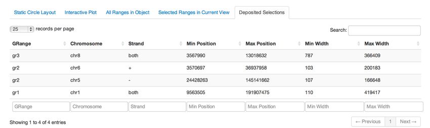
interactiveDisplay: A package for enabling interactive visualization of Bioconductor objects                        8

5.1.5   Plots

                                            Figure 5: Static Circle Layout

The Static Circle Layout is a ggbio [11] based plot is provided for overview purposes and is not intended to represent
the user’s current subsetting operations. It provides the user with a broad summary of the data they submitted in its
unaltered form.

                                              Figure 6: Interactive Plot
interactiveDisplay: A package for enabling interactive visualization of Bioconductor objects 9
The Interactive Plot is the main view for these two methods. Trackplots are drawn with the Bioconductor package
Gviz [3].
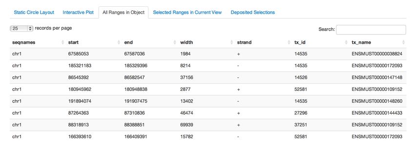
Figure 7: All Ranges in Object
Using Shiny’s advanced datatables, this is a searchable, sortable table of all ranges contained in the current GRanges. In
the case of the GRanges method, this table contains all ranges in the object, and in the GRangesList method the table
contains ranges in the current active GRanges selected from the dropdown.
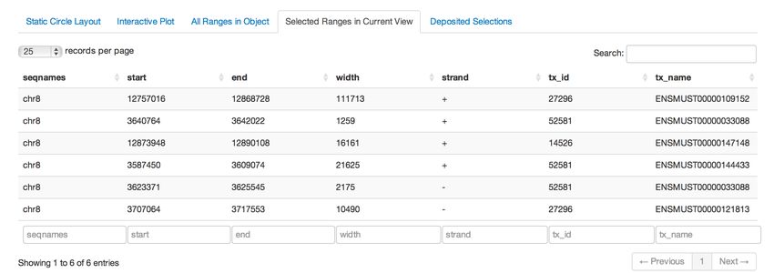
Figure 8: Selected Ranges in Current View
This table is similar to the previous view, except it reflects the current state of subsetting operations performed by the
UI and what is currently displayed in the trackplot.
Figure 9: Deposited Selections
This table view doesn’t show individual ranges, instead it gives a summary of selected ranges that have been locked in
with the Deposit Ranges in View button. Here the user can keep track of sets of ranges of interest that can be sent
back to the console when the application is closed.interactiveDisplay: A package for enabling interactive visualization of Bioconductor objects 10
5.1.6 Metadata Tabset
Figure 10: Dynamically Created Metadata Tabs
The lower tabset consists of individual tabs that are dynamically produced based on the metadata contents of the object
submitted. Each tab has a list of checkboxes that allow the user to subset the selection based on the metadata. The
subsetting is applied across all deposited selections. The usefulness of this panel really depends on the content of the
object submitted. Objects containing no metadata columns obviously have no use for this UI, but metadata rich objects
with categorical, biologically relevant labels can potentially be subset quickly according to them.
5.2 ExpressionSet
5.2.1 Object Background
The ExpressionSet class is a standardized container for gene expression data, specifically from a microarray.
data(expr)
expr
## ExpressionSet (storageMode: lockedEnvironment)
## assayData: 500 features, 26 samples
## element names: exprs, se.exprs
## protocolData: none
## phenoData
## sampleNames: A B ... Z (26 total)
## varLabels: sex type score
## varMetadata: labelDescription
## featureData: none
## experimentData: use 'experimentData(object)'
## Annotation: hgu95av2
We can view the expression values with the exprs() function.
exprs(expr)[1:10,1:7]
## A B C D E F
## AFFX-MurIL2_at 192.7420 85.75330 176.7570 135.57500 64.49390 76.35690
## AFFX-MurIL10_at 97.1370 126.19600 77.9216 93.37130 24.39860 85.50880
## AFFX-MurIL4_at 45.8192 8.83135 33.0632 28.70720 5.94492 28.29250
## AFFX-MurFAS_at 22.5445 3.60093 14.6883 12.33970 36.86630 11.25680
## AFFX-BioB-5_at 96.7875 30.43800 46.1271 70.93190 56.17440 42.67560
## AFFX-BioB-M_at 89.0730 25.84610 57.2033 69.97660 49.58220 26.12620
## AFFX-BioB-3_at 265.9640 181.08000 164.9260 161.46900 236.97600 156.80300
## AFFX-BioC-5_at 110.1360 57.28890 67.3980 77.22070 41.34880 37.97800interactiveDisplay: A package for enabling interactive visualization of Bioconductor objects 11
## AFFX-BioC-3_at 43.0794 16.80060 37.6002 46.52720 22.24750 61.64010
## AFFX-BioDn-5_at 10.9187 16.17890 10.1495 9.73639 16.90280 5.33328
## G
## AFFX-MurIL2_at 160.5050
## AFFX-MurIL10_at 98.9086
## AFFX-MurIL4_at 30.9694
## AFFX-MurFAS_at 23.0034
## AFFX-BioB-5_at 86.5156
## AFFX-BioB-M_at 75.0083
## AFFX-BioB-3_at 211.2570
## AFFX-BioC-5_at 110.5510
## AFFX-BioC-3_at 33.6623
## AFFX-BioDn-5_at 25.1182
The structure of the ExpressionSet object [4]:
expression data (assayData)
sample metadata (phenoData)
annotations and instrument metadata (featureData, annotation)
sample protocol (protocolData)
experimental design (experimentData)
5.2.2 Method
display(expr)
5.2.3 UI
The method for ExpressionSet has the most features of any of the current objects handled by interactiveDisplay. The main
panel consists of three tabs that visualize the data as a heatmap, network and dendrogram. Gene ontology summaries of
probes or selected probe clusters are available in tables in the lower tabset of the main panel.
Figure 11: Experiment Info
The Experiment Info table at the top of the sidebar is entirely dependent on whether the ExpressionSet object submitted
has these fields filled out.
Figure 12: Suppress Heatmap checkbox, Transpose Heatmap checkbox
Depending on whether the parameter sflag=FALSE is passed to the the display() method and the selected dimensions of
the ExpressionSet, replotting the heatmap can introduce delays. Using the checkbox to suppress the heatmap plottinginteractiveDisplay: A package for enabling interactive visualization of Bioconductor objects 12
can circumvent this. Also, depending on the relative dimensions of probes/samples, transposing the plot can make better
use of the space available.
Figure 13: Network/Dendrogram View dropdown
This UI element simply toggles between displaying plots that represent distances/clustering across probes or samples.
Figure 14: Group Wide GO Summary UI
This set of UI elements can be used to provide a gene ontology summary of a chosen cluster of probes in the network
view. Simply mouseover a node within a cluster of interest and the cluster number will pop-up. Input that cluster number
into the input field and hit the View/Update GO Summary button. This can take 10-30 seconds, which is why this is
not automatically reactive. Adjusting the Minimum probe population for GO term allows the user to explore general or
specific top ranking terms. The summary table is located in the second tab of the lower tabset.
Figure 15: Individual Probe GO Summary dropdown
This drop-down contains options from the current subset of probes being visualized. Selecting a probe refreshes the first
tab of the lower tabset with a GO summary for that probe, as well as associated gene names and Entrez IDs. When
toggled to probe view, clicking on a probe node in the network view also refreshes this selection and may be more
convenient.
Figure 16: Subset UIinteractiveDisplay: A package for enabling interactive visualization of Bioconductor objects 13
This UI set is used for subsetting the submitted ExpressionSet object. The initial values are set to the maximum number
of samples and to a very conservative 20 probes. The user is free to expand out to the full dimensions.
Figure 17: Tweak Axis Label Font Size slider
Depending on the dimensions of the ExpressionSet object submitted/subset, it may be necessary to adjust label sizes to
prevent label overlapping or illegibly small text.
Figure 18: Edge/Distance UI
This UI element is used in the network view, allowing the user to determine the number of edges and the distance
threshold represented in the graph.
Figure 19: Force Layout sliders
This is a cosmetic control for the force directed graph, which allows the user to adjust how nodes spread themselves out
and the length of their edges.
Figure 20: Clustering UI
These controls set the parameters for the distance and hierarchical clustering methods used. Only base R methods are
currently implemented but more may be included in future releases as well as possible option of allowing the user to
manually provide their own via a textbox element.interactiveDisplay: A package for enabling interactive visualization of Bioconductor objects 14
Figure 21: Color Picker UI
These elements affect the coloration of the heatmap. The color picker for the tricolor scale is not provided by the Shiny
framework. This uses an additional JavaScript library which will be discussed in a later section. This is not just a cosmetic
option, different modes can better visualize different data and accommodate color blind users.
Figure 22: Stop Application button
This stops the application. The ExpressionSet method does not currently return any data back to the R console.
5.2.4 Plots
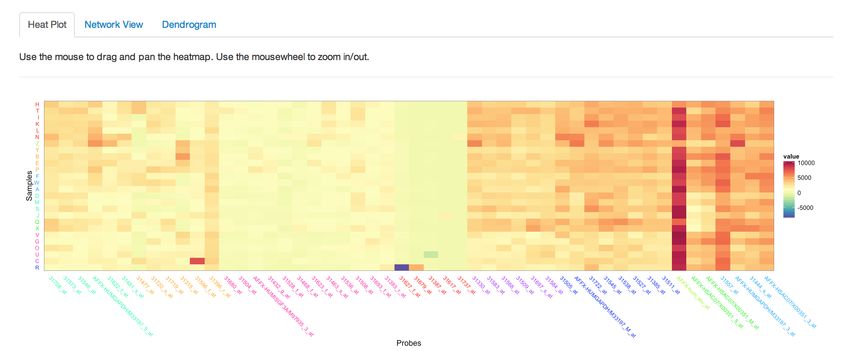
Figure 23: Heat Plot
Many packages on CRAN and Bioconductor have specialized heatmap functions, HeatPlus [6] has a specific function for
ExpressionSet objects. Given that one of the goals of this package is modularity and reuse of code, the more generic
plotting package ggplot2 [10] was used instead of other options. Often heatmap and dendrogram plots are paired together
but given that there is a great deal of screen real estate taken up by tables, UI controls and on-screen documentation,
the dendrograms are moved to a separate tab.interactiveDisplay: A package for enabling interactive visualization of Bioconductor objects 15
Figure 24: Network View - Samples
Figure 25: Network View - ProbesinteractiveDisplay: A package for enabling interactive visualization of Bioconductor objects 16
The Network View uses a D3.js based force directed graph to visualize distance/similarity between samples or probes
based on user selected distance methods and threshold settings. Nodes in the graph are colored based on cluster settings.
As stated previously, when the view is toggled to display probes, there is the added interface functionality of being to
use the graph to conveniently gather GO information. When used in conjunction with the heatmap view, the network
graph can quickly convey to the user which samples have similar profiles or which probes have similar expression across
samples.
Figure 26: Dendrogram - Samples
Figure 27: Dendrogram - Probes
The decision to separate the dendrogram plots from the heatmap was a difficult one, paired heatmap/dendrogram plots
quickly convey clustering groupings alongside the data that they were generated from. However, due to the forementioned
design/layout constraints, dendrograms are placed in their own tab. This keeps the already complex UI as clean as possible
with adequate space for all plots. To accommodate this decision some care was taken to keep some consistency between
views. The clustering colors are consistent across the three views and the sample/probe order is the same between the
heatmap and dendrogram views. This consistency helps the user quickly switch between tabs and stay oriented with the
data they are examining.
5.2.5 GO TabsetinteractiveDisplay: A package for enabling interactive visualization of Bioconductor objects 17
Figure 28: Individual Probe GO Summary
These summary tables provide Entrez ID and gene names for the selected probe and the top ranking results for GO
descriptors. This table allows the user to manually choose and characterize probes that could be exhibiting differential
expression in the submitted espressionSet.
Figure 29: Probe Cluster GO Summary
This tab provides a table of the results of the hyperg() function from the GOstats package [2]. Ranked in order of p-value,
the results give a general GO summary across the group of selected probes. Much like the previous table, this provides
an interactive tool for characterizing differentially expressed sets of probes.interactiveDisplay: A package for enabling interactive visualization of Bioconductor objects 18 5.3 RangedSummarizedExperiment 5.3.1 Object Background data(se) se ## Loading required package: SummarizedExperiment ## Loading required package: MatrixGenerics ## Loading required package: matrixStats ## ## Attaching package: ’matrixStats’ ## The following objects are masked from ’package:Biobase’: ## ## anyMissing, rowMedians ## ## Attaching package: ’MatrixGenerics’ ## The following objects are masked from ’package:matrixStats’: ## ## colAlls, colAnyNAs, colAnys, colAvgsPerRowSet, colCollapse, ## colCounts, colCummaxs, colCummins, colCumprods, colCumsums, ## colDiffs, colIQRDiffs, colIQRs, colLogSumExps, colMadDiffs, ## colMads, colMaxs, colMeans2, colMedians, colMins, colOrderStats, ## colProds, colQuantiles, colRanges, colRanks, colSdDiffs, colSds, ## colSums2, colTabulates, colVarDiffs, colVars, colWeightedMads, ## colWeightedMeans, colWeightedMedians, colWeightedSds, ## colWeightedVars, rowAlls, rowAnyNAs, rowAnys, rowAvgsPerColSet, ## rowCollapse, rowCounts, rowCummaxs, rowCummins, rowCumprods, ## rowCumsums, rowDiffs, rowIQRDiffs, rowIQRs, rowLogSumExps, ## rowMadDiffs, rowMads, rowMaxs, rowMeans2, rowMedians, rowMins, ## rowOrderStats, rowProds, rowQuantiles, rowRanges, rowRanks, ## rowSdDiffs, rowSds, rowSums2, rowTabulates, rowVarDiffs, rowVars, ## rowWeightedMads, rowWeightedMeans, rowWeightedMedians, ## rowWeightedSds, rowWeightedVars ## The following object is masked from ’package:Biobase’: ## ## rowMedians ## class: RangedSummarizedExperiment ## dim: 14599 4 ## metadata(0): ## assays(1): '' ## rownames(14599): FBgn0000003 FBgn0000008 ... FBgn0261574 FBgn0261575 ## rowData names(8): id baseMean ... pval padj ## colnames(4): untreated3 untreated4 treated2 treated3 ## colData names(1): Condition The RangedSummarizedExperiment class is similar to a dataframe where rows represent ranges (using GRanges/GRangesList) and columns represent samples (with sample data summarized as a dataframe). It can contain one or more assays. Ranges have read counts associated with them [4].
interactiveDisplay: A package for enabling interactive visualization of Bioconductor objects 19
5.3.2 Method
display(se)
5.3.3 UI
Figure 30: RangedSummarizedExperiment UI
The UI for the RangedSummarizedExperiment method is relatively simple. It is the best candidate of the existing
methods for future development. The RangedSummarizedExperiment class is widely used, data rich object and has a lot
of potential for improvement.
5.3.4 Plot
Figure 31: Binned Mean Counts by Position
Currently the plot gives a simple depiction of expression score/counts across regions of the selected chromosome. However,
this plot currently obfuscates the relative coverage of the ranges of interest. It will likely need to be replaced with a
multiple track plot in future releases.
6 Additional Functions/Methods
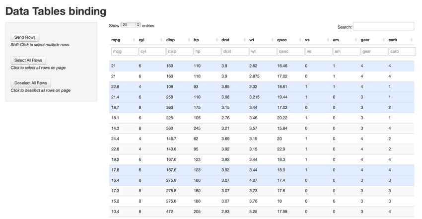
6.1 Dataframe - display()
display(mtcars)
Similar to the GRanges and GRangesList methods, the dataframe method can send a subset of the submitted object back
to the console and can be stored in a new variable.interactiveDisplay: A package for enabling interactive visualization of Bioconductor objects 20 new_mtcars
interactiveDisplay: A package for enabling interactive visualization of Bioconductor objects                           21

6.3    gridsvgjs()
One of the goals of this package is to provide users and future contributors with simple, modular functions that can be
inserted into more complex methods or serve as the foundation or inspiration for future components. This motivation was
behind the decision to export the helper function gridsvgjs(). This function takes any grid based plot, converts it to SVG
format (see section on gridSVG), inserts JavaScript for the Pan/Zoom functionality (see JavaScript Libraries section) and
initiates a local Shiny instance. The four display() methods make use of the majority of the code in gridsvgjs(). After
considering the potential usefulness of doing this with any plot, I repackaged the code as a stand-alone function. The
standard R graphics viewer can sometimes be restrictive, particularly for larger plots. Viewing a plot as a vector based
rendering with pan and zoom capabilities seemed to be a desirable addition to the package. The inserted JavaScript
functionality is relatively simple, but hopefully it will encourage more interactivity in the future.
data(mtcars)
qp
interactiveDisplay: A package for enabling interactive visualization of Bioconductor objects                         22

                                                Figure 34: gridSVG [5]

8     JavaScript Libraries
8.1    Data-Driven Documents
Michael Bostock’s JavaScript library, D3.js (http://d3js.org/), allows for highly customizable data visualizations using
universal web standards. It can work along with Shiny to bind data to the Document Object Model (DOM). Unlike Shiny
which handles the interactive elements but leaves R to handle the visualization, D3.js can handle both. Currently only
the ExpressionSet method’s Network View makes use of this library.

8.2    Zoom/Pan JavaScript libraries
This Zoom/Pan library is used in all four main display() methods and in gridsvgjs(). While a relatively simple feature,
hopefully it will lead to more complex JavaScript interactivity that directly manipulates plots produced by R plotting
packages. The Andrea Leofreddi’s original JavaScript code was expanded upon by John Krauss to produce the version
of this library used in interactiveDisplay.
Andrea Leofreddi
https://code.google.com/p/svgpan/
John Krauss
https://github.com/talos/jquery-svgpan

8.3    JavaScript Color Chooser
The colorpicker included in the ExpressionSet method should eventually be moved into the Shiny package itself. Many
R users outside of the Bioconductor community use RColorBrewer and could make use of this UI element in their Shiny
based applications.
Jan Odvarko
http://jscolor.com/

9     Acknowledgments
Shiny
Joe Cheng and Winston Chang
http://www.rstudio.com/shiny/
Force Layout
Jeff Allen
https://github.com/trestletech/shiny-sandbox/tree/master/grn
interactiveDisplay: A package for enabling interactive visualization of Bioconductor objects 23 gridSVG Simon Potter http://sjp.co.nz/projects/gridsvg/ Zoom/Pan JavaScript libraries John Krauss https://github.com/talos/jquery-svgpan Andrea Leofreddi https://code.google.com/p/svgpan/ JavaScript Color Chooser Jan Odvarko http://jscolor.com/ Data-Driven Documents Michael Bostock http://d3js.org/ 10 SessionInfo sessionInfo() ## R Under development (unstable) (2021-02-10 r79979) ## Platform: x86_64-pc-linux-gnu (64-bit) ## Running under: Ubuntu 20.04.2 LTS ## ## Matrix products: default ## BLAS: /home/biocbuild/bbs-3.13-bioc/R/lib/libRblas.so ## LAPACK: /home/biocbuild/bbs-3.13-bioc/R/lib/libRlapack.so ## ## locale: ## [1] LC_CTYPE=en_US.UTF-8 LC_NUMERIC=C ## [3] LC_TIME=en_US.UTF-8 LC_COLLATE=C ## [5] LC_MONETARY=en_US.UTF-8 LC_MESSAGES=en_US.UTF-8 ## [7] LC_PAPER=en_US.UTF-8 LC_NAME=C ## [9] LC_ADDRESS=C LC_TELEPHONE=C ## [11] LC_MEASUREMENT=en_US.UTF-8 LC_IDENTIFICATION=C ## ## attached base packages: ## [1] stats4 grid parallel stats graphics grDevices utils ## [8] datasets methods base ## ## other attached packages: ## [1] SummarizedExperiment_1.21.1 MatrixGenerics_1.3.1 ## [3] matrixStats_0.58.0 GenomicRanges_1.43.3 ## [5] GenomeInfoDb_1.27.7 IRanges_2.25.6 ## [7] S4Vectors_0.29.7 Biobase_2.51.0 ## [9] interactiveDisplay_1.29.1 BiocGenerics_0.37.1 ## [11] ggplot2_3.3.3 knitr_1.31 ## ## loaded via a namespace (and not attached): ## [1] httr_1.4.2 bit64_4.0.5 ## [3] jsonlite_1.7.2 splines_4.1.0 ## [5] shiny_1.6.0 assertthat_0.2.1 ## [7] interactiveDisplayBase_1.29.0 highr_0.8
interactiveDisplay: A package for enabling interactive visualization of Bioconductor objects                      24

##    [9]   RBGL_1.67.0                       blob_1.2.1
##   [11]   GenomeInfoDbData_1.2.4            Category_2.57.2
##   [13]   pillar_1.5.1                      RSQLite_2.2.3
##   [15]   lattice_0.20-41                   glue_1.4.2
##   [17]   digest_0.6.27                     RColorBrewer_1.1-2
##   [19]   promises_1.2.0.1                  XVector_0.31.1
##   [21]   colorspace_2.0-0                  htmltools_0.5.1.1
##   [23]   httpuv_1.5.5                      Matrix_1.3-2
##   [25]   plyr_1.8.6                        GSEABase_1.53.1
##   [27]   XML_3.99-0.5                      pkgconfig_2.0.3
##   [29]   genefilter_1.73.1                 zlibbioc_1.37.0
##   [31]   purrr_0.3.4                       xtable_1.8-4
##   [33]   scales_1.1.1                      later_1.1.0.1
##   [35]   tibble_3.1.0                      annotate_1.69.0
##   [37]   KEGGREST_1.31.1                   generics_0.1.0
##   [39]   ellipsis_0.3.1                    cachem_1.0.4
##   [41]   withr_2.4.1                       survival_3.2-7
##   [43]   magrittr_2.0.1                    crayon_1.4.1
##   [45]   mime_0.10                         memoise_2.0.0
##   [47]   evaluate_0.14                     fansi_0.4.2
##   [49]   graph_1.69.0                      tools_4.1.0
##   [51]   lifecycle_1.0.0                   stringr_1.4.0
##   [53]   munsell_0.5.0                     DelayedArray_0.17.9
##   [55]   AnnotationDbi_1.53.1              Biostrings_2.59.2
##   [57]   compiler_4.1.0                    rlang_0.4.10
##   [59]   debugme_1.1.0                     RCurl_1.98-1.2
##   [61]   bitops_1.0-6                      gtable_0.3.0
##   [63]   DBI_1.1.1                         reshape2_1.4.4
##   [65]   R6_2.5.0                          dplyr_1.0.5
##   [67]   fastmap_1.1.0                     bit_4.0.4
##   [69]   utf8_1.1.4                        gridSVG_1.7-2
##   [71]   stringi_1.5.3                     Rcpp_1.0.6
##   [73]   vctrs_0.3.6                       png_0.1-7
##   [75]   tidyselect_1.1.0                  xfun_0.21

11      References
 [1] Marc Carlson and Sonali Arora. AnnotationHub: A client for retrieving Bioconductor objects from AnnotationHub.
     R package version 1.4.0.
 [2] S Falcon and R Gentleman. Using GOstats to test gene lists for GO term association. Bioinformatics, 23(2):257–8,
     2007.
 [3] Florian Hahne, Steffen Durinck, Robert Ivanek, Arne Mueller, Steve Lianoglou, and Ge Tan. Gviz: Plotting data
     and annotation information along genomic coordinates. R package version 1.8.2.
 [4] Michael Lawrence, Wolfgang Huber, Hervé Pagès, Patrick Aboyoun, Marc Carlson, Robert Gentleman, Martin
     Morgan, and Vincent Carey. Software for computing and annotating genomic ranges. PLoS Computational Biology,
     9, 2013.
 [5] Paul Murrell and Simon Potter. gridSVG: Export grid graphics as SVG, 2013. R package version 1.4-0.
 [6] Alexander Ploner. Heatplus: Heatmaps with row and/or column covariates and colored clusters, 2014. R package
     version 2.11.0.
interactiveDisplay: A package for enabling interactive visualization of Bioconductor objects 25
[7] R Core Team. R: A Language and Environment for Statistical Computing. R Foundation for Statistical Computing,
Vienna, Austria, 2013.
[8] RStudio and Inc. shiny: Web Application Framework for R, 2014. R package version 0.9.1.
[9] Deepayan Sarkar. Lattice: Multivariate Data Visualization with R. Springer, New York, 2008. ISBN 978-0-387-
75968-5.
[10] Hadley Wickham. ggplot2: elegant graphics for data analysis. Springer New York, 2009.
[11] Tengfei Yin, Dianne Cook, and Michael Lawrence. ggbio: an r package for extending the grammar of graphics for
genomic data. Genome Biology, 13(8):R77, 2012.You can also read