Predicting Elections for Multiple Countries Using Twitter and Polls
←
→
Page content transcription
If your browser does not render page correctly, please read the page content below
This article has been accepted for publication in IEEE Intelligent Systems but has not yet been fully edited.
                                       Some content may change prior to final publication.

    Predicting Elections for Multiple Countries Using Twitter and Polls
         Adam Tsakalidis1,2, Symeon Papadopoulos1, Alexandra Cristea2, Yiannis Kompatsiaris1
     1
      Information Technologies Institute, Center for Research and Technology Hellas
     Thessaloniki, Greece
     {atsak,papadop,ikom}@iti.gr

     2
      Department of Computer Science, University of Warwick
     Coventry, UK
     {a.tsakalidis,a.i.cristea}@warwick.ac.uk

                                                Abstract
Our work focuses on predicting the 2014 European Union elections in three different countries, using
Twitter and polls. Past works on this domain relying strictly on Twitter data have been proven
ineffective. Others, using polls as their ground-truth, have raised questions regarding the contribution
of Twitter data for this task. Lastly, most works provide their results after the end of the elections and
hence are possibly biased. Here, we treat this task as a multivariate time series forecast; we extract
Twitter- and poll-based features and train different predictive algorithms, releasing the results for one
country before the end of the elections. We achieve better results than several past works and
commercial baselines and, most importantly, we demonstrate the significant effectiveness of Twitter
data for this task.

Keywords: Machine learning; Web mining; Twitter; elections; time series forecasting

1 Introduction
Twitter is a microblogging social platform, which has seen an amplified overall interest, recording
about 500 million short messages sent per day (https://about.twitter.com/company). Hence, it is not
surprising that it is increasingly exploited for various research tasks, including modelling and
predicting users’ behaviour.
The current work focuses on exploiting its content for the task of predicting the 2014 European Union
(EU) Election results in Germany, the Netherlands and Greece. While several works have been
conducted on the same domain, many of them relied strictly on Twitter data and have been proven
ineffective when tested in different elections. Furthermore, most of the past works have published their
results after the elections; others raised questions on the benefit of using Twitter data for this task [8].
In this work, we treat the users’ voting intentions as time-variant features. Instead of trying to predict
every user’s vote, we treat Twitter political discussions as a general index that varies with time; we
define several Twitter-based features and fit them in time-series models, using opinion polls as our
ground-truth. In this way, we combine the Twitter-based time-series with the poll-based ones. We test
three different forecasting algorithms using three different sets of features; we contrast our results with
several popular methods, achieving lower error rates even compared to prediction websites and polls.
Furthermore, working on different elections at the same time, we demonstrate the portability of our
approach. Most importantly though, we show that by using the proposed Twitter-based features, all
tested algorithms get a significant boost in accuracy, compared to when using only poll-based features.
Last but not least, we are among the first to have published our predictions before the announcement of
the Exit Polls for one country (Greece, http://socialsensor.eu/news/132-socialsensor-eu-elections-
predictions), preventing any bias towards them, while we follow the exact same methodology for the
other two countries.

                       Digital Object Indentifier 10.1109/MIS.2015.17          0885-9000/$26.00 2015 IEEE
This article has been accepted for publication in IEEE Intelligent Systems but has not yet been fully edited.
Some content may change prior to final publication.
2 Background
2.1 EU Elections
The EU Parliament elections are held every five years among the EU member states. Elections take
place almost simultaneously across Europe and people vote for the national parties of their countries.
The 2014 EU elections were judged as extremely important, in light of the economic crisis and the rise
of Euroscepticism. Due to the nature of these elections, it is difficult to predict the results at a pan-
European level without taking into account the important demographic and political differences
between the EU members. Thus, we focused on three different countries, transferring the problem to a
national level. The elections were held on May, 22 for the Netherlands and on May, 25 for Germany
and Greece. There were 10 main political parties contesting in the Netherlands, 6 in Germany and 8 in
Greece.
2.2 Related Work
A seminal work on the problem of predicting election results was performed by Tumasjan et al. [10],
demonstrating that the number of times the name of a political party appears on Twitter is a fairly good
estimate of its voting share. However, their method was not generalisable to other cases [1]. Naïve
counting and sentiment analysis methods did not perform well either: [4] predicted the correct result,
with two candidates, in only half of the cases.
Recent Twitter-based works use opinion polls as ground-truth. Lei et al. [9] used aggregated poll
reports to train their Twitter-based models, by also examining the geographical locations of the users in
an attempt to predict the results per-location. However, sentiment analysis features, which are
considered to be important for this task, were not included in their modelling. Using poll reports as
ground-truth, Lampos et al. [3] created time-series by taking into account both user- and keyword-
based features for the major parties of two countries; however, their evaluation is performed against
pollsters and not the actual results. Sang and Bos tuned their Twitter-based data on polls, achieving
however slightly worse results [8]. More disturbingly, when they replaced their Twitter-based features
with uniform variables, their predictions got better, implying that Twitter did not actually help in the
prediction task. For a more complete review of the field, the reader is prompted to the work of Gayo-
Avello [2].
3 Methodology
Approaching our problem as a multivariate time-series forecasting task for each country separately, we
create time-series of 11 Twitter- and one poll-based features for every party (sections 3.2-3.3). An
example is the number of tweets mentioning a certain party on a specific day (Twitter-based) and the
percentage for that party reported on a poll that was conducted on that day (poll-based). Next, we
provide all these features as input to different forecasting algorithms for predicting the voting share of
every party separately (section 3.4).
3.1 Data Aggregation
We started aggregating data published on Twitter and various opinion polls on a per-country basis from
April, 6th until two days before the elections (20/5 for the Netherlands and 23/5 for Germany and
Greece), leaving one day to conduct our processing. Using the public Twitter Streaming API
(https://dev.twitter.com/), we aggregated tweets written in the respective language that contained a
party’s name, its abbreviation, its Twitter account name and some possible misspellings (e.g., grunen
instead of grünen). We excluded several ambiguous keywords in order to reduce noise (e.g., the
abbreviation of the Dutch party “GL” may stand for “good luck”), which might slightly affect the
Digital Object Indentifier 10.1109/MIS.2015.17 0885-9000/$26.00 2015 IEEEThis article has been accepted for publication in IEEE Intelligent Systems but has not yet been fully edited.
Some content may change prior to final publication.
replication of naïve counting-based methods. The aggregated tweet ids are available at
http://mklab.iti.gr/project/eu-elections-2014-prediction-dataset.
3.2 Modelling
Twitter Features: We extract several Twitter-based features potentially disclosing the users’ voting
intentions. These features were based on past works, showing that the counts of a political party on
Twitter and the expressed sentiment towards it are – to some extent – related with its voting share in the
elections. However, instead of relying strictly on counting-based methods, we incorporate daily
features into time-series, in order to correlate them to the opinion polls (discussed next).
Working on every country separately, we first assigned equal weights to all parties mentioned in a
tweet, so that they sum up to one. Let td(p) denote the (weighted) number of tweets that mention party p
on day d and tposd(p) (tnegd(p)) the corresponding number of tweets containing positive (negative)
content. Similarly, let ud(p) denote the number of users mentioning party p on day d and uposd(p)
(unegd(p)) the number of users that have published a tweet with positive (negative) content about party
p on that day. We constructed the following features, for every day:
Feature Definition
numTweetsd ݐௗ ሺ݅ሻ
ݐௗ ሺሻ
pctTweetsd(p)
σ ݐௗ ሺ݅ሻ
ݏݐௗ ሺሻ
pctTPosd(p)
ݐௗ ሺሻ
݃݁݊ݐௗ ሺሻ
pctTNegd(p)
ݐௗ ሺሻ
ݏݐௗ ሺሻ
pctTPosShared(p)
σ ݏݐௗ ሺ݅ሻ
݃݁݊ݐௗ ሺሻ
pctTNegShared(p)
σ ݃݁݊ݐௗ ሺ݅ሻ
ݑௗ ሺሻ
pctUsersd(p)
σ ݑௗ ሺ݅ሻ
ݏݑௗ ሺሻ
pctUPosd(p)
ݑௗ ሺሻ
݃݁݊ݑௗ ሺሻ
pctUNegd(p)
ݑௗ ሺሻ
σௗ௫ୀ ݑ௫ ሺሻ
pctTotalUsersd(p)
σௗ௫ୀ σ ݑ௫ ሺ݅ሻ
Here, pctTotalUsersd(p) refers to the distinct number of the users that have mentioned p, divided by the
total number of users up to day d. We also added the average sentiment value (avgSentimentd) as an
eleventh feature (notice that numTweetsd and avgSentimentd were the same for all parties within a
country). Finally, we used a 7-day Moving Average (MA) filter for all features (except
pctTotalUsersd(p)) in order to normalise their values, as suggested by O’Connor et al. [6]. These 11
Digital Object Indentifier 10.1109/MIS.2015.17 0885-9000/$26.00 2015 IEEEThis article has been accepted for publication in IEEE Intelligent Systems but has not yet been fully edited.
Some content may change prior to final publication.
values for every party were used as our Twitter-based features and were provided as input to our
algorithms, along with the opinion poll ones.
Opinion Polls: Since there is not a complete polling aggregation service, we had to find different polls
manually. Once aggregated, we removed all poll values from “small” parties (not appearing in all polls)
and added their voting share to the “Others” bucket, since we were only interested in the main parties
of each country; then, we distributed proportionally to all parties (including “Others”) the voting share
of all “undecided” voters. In this way we managed to have consistent polls, adjusting their reports to
include only the main political parties of each country, along with the “Others”.
While creating time-series of Twitter features without missing values was a straightforward process,
this was not the case for the polls. A poll is usually conducted over two to three days; we treated the
adjusted results as the actual voting shares each party would have received if the elections were held on
any of these days. If two or more polls were held on the same day, we considered the voting share of
each party as the weighted average value, using the sample size of every poll as the weight and making
sure that all voting shares sum up to 100. We then filled all days without polling data by using linear
interpolation. Finally, for the days after the last poll, we replicated the last poll-based value for every
party in order to set the prediction horizon to 1 for our predictive algorithms, for consistency between
the different countries. There was only one such day (that is, the last day) for Germany and the
Netherlands.
3.3 Sentiment Analysis
Several Twitter-based features were sentiment-related; hence, we needed to assign a sentiment value to
each tweet before proceeding. One of the most popular approaches of sentiment analysis is to train a
classifier on a labelled corpus of tweets and apply it to the desired test set. However, past works have
revealed the domain-dependent nature of such classifiers [7]. The integration of Part-of-Speech (POS)
tags is also beneficial, but there does not exist a reliable, free-to-use POS tagger for the three
languages. Given these constraints, we decided to adopt a lexicon-based approach, in order to create a
generic method that could be applied in different cases. While such approaches perform only slightly
better than a random classifier [4], we were only interested in the daily differences of the expressed
sentiment; thus, given that we have enough data on every day, even a slightly better than the random
classifier method could fit our goals [6].
Due to the lack of a sentiment lexicon for different languages, we translated three English lexicons
using Google Translate (https://translate.google.com/). These included SentiWordNet
(http://sentiwordnet.isti.cnr.it/, about 150,000 synsets with a double value indicating their polarity),
Opinion Lexicon (http://www.cs.uic.edu/~liub/FBS/sentiment-analysis.html, about 6,800 polarized
terms) and the Subjectivity Lexicon that serves as part of the Opinion Finder
(http://mpqa.cs.pitt.edu/opinionfinder/, about 8,000 terms along with their Part-of-Speech (POS),
subjectivity – strong/weak – and polarity indication).
We assigned the values of 1 and −1 for the positive and negative terms in the Opinion Lexicon
respectively; for the Subjectivity Lexicon, we used four values (−1, −0.5, 0.5, 1) to represent every
subjective word based on subjectivity (|0.5| for weak, |1| for strong) and polarity; for SentiWordNet,
we kept the values of every synset. We removed all terms that were not a single word, due to the
inaccuracy observed in those translations. If the same word appeared in different lexicons, we
considered the average as its sentiment value, resulting into 14,060/19,357 German, 13,838/18,993
Dutch and 13,582/18,356 Greek positive/negative terms. In order to detect a tweet’s sentiment, we used
a naïve sum-of-weights method on its keywords, according to the respective lexicon, and assigned the
majority class label (positive/negative) to it.
Digital Object Indentifier 10.1109/MIS.2015.17 0885-9000/$26.00 2015 IEEEThis article has been accepted for publication in IEEE Intelligent Systems but has not yet been fully edited.
Some content may change prior to final publication.
3.4 Algorithms
We tested three different algorithms on each political party separately, using only this specific party’s
features (11 Twitter- and one poll-based) as input. These algorithms were Linear Regression, Gaussian
Process and Sequential Minimal Optimization for Regression, all implemented using Weka
(http://www.cs.waikato.ac.nz/ml/weka/) with the default settings (our released results included a fourth
algorithm (Support Vector Regression); due to its poor performance in Greece, we did not test it on the
other countries). Since it was difficult to evaluate each algorithm before the elections, we initially
decided to empirically apply a seven-day training window for every algorithm and considered the
average predicted percentage for every party as our final estimate.
4 Data
4.1 Twitter
We aggregated 361,713 tweets from 74,776 users in Germany, 452,348 from 74,469 users in the
Netherlands and 263,465 from 19,789 users in Greece. Our findings on the average sentiment value
reveal that negative opinions dominate in political discussions (−0.54 for Germany, −1.09 for the
Netherlands and −0.29 for Greece). Figure 1 shows that there were far more tweets published in the
week before the elections, whereas a slight decrease is noticed in the Easter week (13 − 20/4). Still, due
to the restrictions of the Twitter Streaming API (it returns no more than 1% of all public tweets), we
could have missed some data. Research has shown that the increase of global awareness on a topic, or
the sudden decrease in tweets on a day could result into a decrease of the coverage of the Streaming
API and, consequently, lead to a noisy bias [5]. However, since the total amount of aggregated data is
fairly moderate, our data loss (if any) is probably negligible. Moreover, as we are only interested in
time-series modelling, this should not affect our process.
Figure 1: Number of political tweets aggregated per day, after a 7-day MA
4.2 Opinion Polls
In total, we used 26 different polls from 11 diverse sources in Greece, 9 from 4 sources in Germany and
13 polls from 3 sources in the Netherlands. More specifically, we used all the polls published in
Digital Object Indentifier 10.1109/MIS.2015.17 0885-9000/$26.00 2015 IEEEThis article has been accepted for publication in IEEE Intelligent Systems but has not yet been fully edited.
Some content may change prior to final publication.
MetaPolls (http://metapolls.net/); further resources used were http://www.wahlrecht.de/ for Germany,
http://www.3comma14.gr/ for Greece and polls from Ipsos (http://www.ipsos-nederland.nl/), TNS Nipo
(http://www.tns-nipo.com/) and Peil (https://www.noties.nl/peil.nl/) for the Netherlands.
Table 1 shows the variance of every party’s voting share based on all collected poll results, after our
pre-processing (for the Netherlands the “Others” category was missing in most polls and thus not
included in our analysis). The voting shares of the German parties are rather stable, unlike the
percentages reported for the Dutch and the Greek parties, reflecting the differences of people’s voting
intentions through time. Not surprisingly, since polls were part of our training process, we achieved
lower error rates in Germany than the other countries (see next section).
Table 1: Variance of reported shares in the processed polls
Germany The Netherlands Greece
CDU/CSU 1.15 PVV 1.80 ND 3.39
SPD 0.99 VVD 3.88 SYRIZA 4.29
Grünen 1.00 D66 1.41 XA 2.36
Linke 0.63 CDA 3.38 Potami 5.38
AfD 0.25 PvdA 1.85 KKE 0.54
FDP 0.25 SP 2.00 Elia 1.49
Others 1.00 CU/SGP 0.64 ANEL 0.62
GL 0.46 DIMAR 0.36
50+ 0.24 Others 1.95
PvdD 0.40
Average 0.75 Average 1.61 Average 2.51
5 Results
In the current section we present the results obtained from our method (denoted as “Twitter-Poll-
Based”, “TPB”), along with several other competing methods. These were a combination of established
naïve methods, past works, commercial resources and our method when leaving some features out:
x CB1: The Count-Based method by Tumasjan et al. [10].
x CB2: A similar naïve method [8], applied by keeping the tweets that mention only one party
and then the first tweet of every user. At the final stage, voting shares are given to the parties as
in CB1. In both “CB” cases, since we did not have data for the last day before the elections, we
worked on the last seven days that we had data for (for the week ending two days before the
elections).
x SB: This is a replication of the work by Sang & Bos [8]. We train on all polls before the last
week. For sentiment analysis, we use our own naïve dictionary-based method. In the original
paper, sentiment values are given to the parties after manual annotation of some tweets.
Nevertheless, these sentiment values are then adjusted to the “population weights”, so our
sentiment analysis choice should not affect the results.
x Polls: The average of the polls conducted during the last processing week; due to the different
companies publishing their poll results at the same time, we provide the average of their reports.
There was one poll in Germany, two in the Netherlands and seven in Greece.
Digital Object Indentifier 10.1109/MIS.2015.17 0885-9000/$26.00 2015 IEEEThis article has been accepted for publication in IEEE Intelligent Systems but has not yet been fully edited.
Some content may change prior to final publication.
x MP: This baseline refers to the predictions of MetaPolls. To the best of our knowledge, this is
one of the only two websites providing predictions for all EU countries. MetaPolls provide their
voting estimates for every party in a range of values; we considered the average value of this
range for every party as the predicted percentage, making sure that the values sum up to 100.
x PW: Similarly, PollWatch (http://www.electio2014.eu/) is the official prediction website that is
powered by VoteWatch Europe and Burson-Marsteller/Europe Decides.
x PB: In order to evaluate the use of our Twitter features, we compare against using only polling
data as features. Hence, this Poll-Based method averages our three algorithms from section 3.4,
fed only with poll-based data.
x CPB: Similarly, the “Counting-Poll-Based” method was used to evaluate the performance of
our sentiment analysis features. Hence, its features include the polling data points along with all
the non-sentiment Twitter features (numTweets, pctTweets, pctUsers, pctUsersTotal).
In order to evaluate both the voting share predictions of the competing methods and the ranking of the
parties, we selected the standard Mean Absolute Error (MAE), the Mean Squared Error (MSE) and the
Tau Kendall Coefficient (τα) as our evaluation metrics. Table 2 presents all the results together, along
with the average per-country values of our evaluation metrics.
As expected, naïve methods perform the worst. While in [8] CB2 provided a boost in accuracy
compared to CB1 against polls, our findings show that this accuracy drops against the actual results.
Surprisingly though, these approaches are the most successful for certain parties – CB2 is the best
method for 4/26 parties; despite that, it is the worst method overall.
SB fails to perform competitively compared to other approaches. Whilst this might be influenced by the
different sentiment analysis method used, it mainly suggests the importance of computing people’s
voting intentions as time-variant features, instead of as static values.
Polls error values vary a lot among the three different countries. In Germany, Polls was the second best
predictor for the final result, in terms of MAE. However, in both Greece and the Netherlands, it
performed relatively poorly, compared to other poll-based methods. This is an interesting point:
although our models (TPB, PB, CPB) used polls for training, they manage to outperform Polls in both
error metrics, by using knowledge from the past. Given that every poll has a standard error (usually
around 3%) along with a certain number of undecided voters, treating polls (next to other features) as
time-series seems a better practice. Overall, only two (out of ten) polls conducted during the last week
achieved better results in MAE than our TPB approach (one in Greece, with MAE 1.35, and one in the
Netherlands, with MAE 1.78). Moreover, Polls have the second highest τα value; however, the
differences among most models are minor. From the two prediction websites, MP outperformed PW by
a margin of 0.33 in MAE. The most likely reason for this big difference is that MP released their
predictions one day before the elections, whereas PW published them on 20/5 for all countries.
Overall, our TPB model performed the best in both error rate terms. However, it did not perform
equally well in terms of correct ranking of the parties, following by 0.03 the best competing model
(PB) in τα. One possible explanation of this effect is that, as we were not interested in correctly ranking
the political parties, but instead predicted their voting shares individually, only the features related to an
individual party were used for the prediction for this party. Using features from different parties in
order to predict each party’s voting share is a challenging task for future research.
From the three algorithms used in TPB – not presented in Table 2 due to space limitations –, Gaussian
Process achieved the lowest MAE (1.31), followed by Sequential Minimal Optimization (1.35) and
Linear Regression (1.42). This means that Gaussian Process performed better than our “averaging”
TPB model. However, since we did not know how reliable the polls were, we did not have a guaranteed
Digital Object Indentifier 10.1109/MIS.2015.17 0885-9000/$26.00 2015 IEEEThis article has been accepted for publication in IEEE Intelligent Systems but has not yet been fully edited.
Some content may change prior to final publication.
ground-truth before the elections and the “averaging” method seemed a safer choice.
Importantly, the comparisons between TPB and PB (and TPB and CPB, respectively) show that our
Twitter features were beneficial. However, the differences between error rates are rather small.
Furthermore, in the case of the Netherlands, PB and CPB achieved better results. So, whilst our
approach achieved the best results overall, the exact contribution of Twitter and sentiment features
needs to be further explored, as follows.
Table 2: Results and predictions per country. The predictions with the lowest MAE per party are in bold.
Party Result CB1 CB2 SB Polls MP PW PB CPB TPB
CDU 35.30 18.38 17.98 33.36 37.50 37.76 37.70 37.51 37.93 37.09
Germany (DE)
SPD 27.30 20.52 17.78 31.74 26.50 26.53 27.00 26.47 26.35 26.87
Grünen 10.70 9.41 10.25 6.67 10.00 10.07 10.70 9.76 9.33 9.82
Linke 7.40 10.25 8.64 7.64 7.50 8.28 8.30 7.22 7.66 7.24
AfD 7.10 23.55 17.91 9.92 7.00 6.58 6.30 7.10 7.08 7.56
FDP 3.40 9.09 18.63 1.87 3.50 3.39 3.00 3.84 3.47 3.38
Others 8.80 – – – 8.00 7.38 7.00 8.10 8.18 8.04
MAE 0.00 8.33 9.10 2.50 0.69 0.96 0.94 0.76 0.85 0.64
DE
MSE 0.00 107.49 123.53 8.36 0.95 1.44 1.53 1.02 1.45 0.71
Tau 1.00 0.20 -0.07 0.60 1.00 0.90 1.00 1.00 1.00 0.90
D66 15.87 14.79 13.58 24.96 17.49 17.68 18.53 16.49 16.22 15.72
The Netherlands (NL)
CDA 15.56 8.73 9.46 13.13 11.84 12.63 11.46 13.33 13.70 13.16
PVV 13.65 14.94 10.80 15.40 16.28 13.64 14.23 15.66 16.09 16.70
VVD 12.32 12.25 11.87 14.58 16.26 13.13 13.92 15.51 15.09 15.51
SP 9.84 17.71 21.30 8.84 12.97 12.32 11.46 13.56 13.28 13.33
PvdA 9.64 13.10 12.35 6.59 7.64 10.00 10.33 6.88 7.28 7.11
CU-SGP 7.86 5.57 7.84 4.22 7.21 9.60 9.32 7.90 7.49 7.77
GL 7.16 7.85 6.96 5.87 4.47 5.25 5.73 4.77 4.91 4.77
PvdD 4.32 4.20 4.39 4.59 3.24 2.22 1.44 3.32 3.40 3.40
50plus 3.78 0.86 1.45 1.80 2.60 3.54 3.58 2.58 2.54 2.52
MAE 0.00 2.66 2.85 2.68 2.26 1.44 1.72 1.91 1.80 1.94
NL
MSE 0.00 13.76 19.50 12.59 6.28 2.99 4.24 4.91 4.22 5.19
Tau 1.00 0.56 0.56 0.82 0.87 0.87 0.85 0.82 0.87 0.78
SYRIZA 26.60 22.55 21.16 23.77 28.60 29.00 29.60 27.72 26.48 27.25
ND 22.71 18.60 15.58 19.77 25.32 25.50 26.00 25.81 23.89 24.67
XA 9.38 14.92 22.71 13.47 9.45 9.40 8.00 10.02 9.45 9.06
Greece (GR)
Elia 8.02 3.99 7.23 6.57 7.13 7.30 6.50 7.40 8.31 8.10
Potami 6.61 4.39 6.24 3.46 7.73 7.70 8.00 6.56 10.73 8.07
KKE 6.07 8.17 7.19 10.02 6.50 6.10 6.00 5.97 6.30 6.16
ANEL 3.47 9.61 2.83 5.38 4.09 4.00 5.10 4.16 3.63 4.26
DIMAR 1.21 1.85 1.13 1.62 2.32 2.40 3.20 2.61 1.90 2.72
Others 15.93 – – – 8.85 8.60 7.60 9.75 9.31 9.71
MAE 0.00 3.60 3.61 2.59 1.77 1.79 2.51 1.55 1.50 1.45
GR
MSE 0.00 15.96 32.56 8.10 7.20 7.85 11.33 5.82 6.98 5.34
Tau 1.00 0.57 0.79 0.79 0.89 0.89 0.82 0.94 0.78 1.00
MAE 0.00 4.87 5.19 2.59 1.57 1.39 1.73 1.40 1.38 1.35
Average
MSE 0.00 45.74 58.53 9.68 4.81 4.10 5.70 3.91 4.21 3.75
Tau 1.00 0.44 0.42 0.74 0.92 0.89 0.89 0.92 0.88 0.89
Digital Object Indentifier 10.1109/MIS.2015.17 0885-9000/$26.00 2015 IEEEThis article has been accepted for publication in IEEE Intelligent Systems but has not yet been fully edited.
Some content may change prior to final publication.
6 Post-hoc Analysis and Discussion
Recall that all of our models (TPB, PB, CPB) were based on a 7-day training window and the average
of the predictions by Linear Regression (LR), Gaussian Process (GP) and Sequential Minimal
Optimization for Regression (SMO) were reported in Table 2. Both of these decisions (window size,
averaging) were made empirically, since we did not know the actual results. In order to better compare
these models, we applied the same algorithms trained on five different window sizes (starting from
one-week with weekly increases of training size up to five-weeks). In this section, we also provide the
results obtained from each individual algorithm (LR, GP, SMO) for every model.
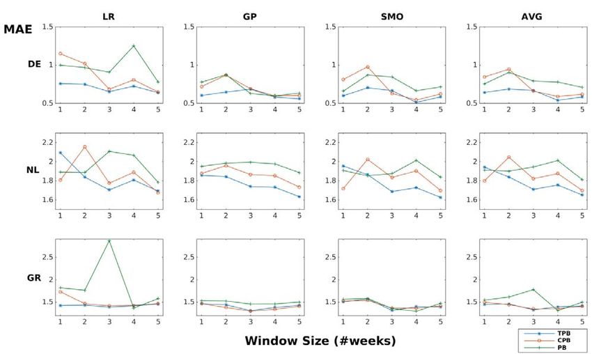
Figure 2 presents the MAE values for all countries and for all algorithms (including our “averaging” –
“AVG” – approach) when trained on different sets of features (leading to TPB, PB, CPB models) and
on different time windows. In most cases, the error drops when we use our complete TPB model’s
features; this holds in 71% of the total cases for the individual algorithms (12/15 for LR and 10/15 for
GP and SMO) and 67% for the “averaging” method (10/15). We also notice that, in most cases, the
errors follow a downwards trend as the training window size increases. Hence, training over a wider
period seems beneficial, although finding the optimal window remains a challenging task for future
research.
On a per-window size, cross-country average, LR performs consistently worse than GP and SMO in all
feature models (the only exception being for TPB in the two-week training window), indicating that it
was a poor choice to include it in our models. The differences between GP and SMO are minor. Using
our TPB model’s features, GP achieves more stable MAE values across different window sizes, ranging
on a cross-country average from 1.21 (5-week) to 1.31 (1-week); however, for the same features, the
best cross-country performance in MAE terms is achieved by SMO (1.20, for the 5-week training
window size).
Figure 2: MAE per training window size for different algorithms and countries
Despite the better overall performance of all algorithms comprising our TPB model, when compared to
PB and CPB (see Figure 2), we need to further test for significant differences between the different
Digital Object Indentifier 10.1109/MIS.2015.17 0885-9000/$26.00 2015 IEEEThis article has been accepted for publication in IEEE Intelligent Systems but has not yet been fully edited.
Some content may change prior to final publication.
models. Thus, we applied the non-parametric Wilcoxon test (two-tailed) to all three algorithms, as well
as our “averaging” initial approach, using the MAEs and MSEs obtained by every algorithm on every
country and training window size.
Comparing TPB and PB revealed that for all three algorithms as well as the “averaging” approach,
there exist significant differences in MAE for the level of .05. The same test of the respective MSEs
revealed significant differences for the .05 level for LR, GP and the “averaging” approach, but not for
SMO (p = .057). Comparing TPB with the CPB MAE rates revealed significant differences for the .05
level for all methods except SMO; for the same level, the differences for all algorithms and our
“averaging” method were significant when applied to the MSE rates. These results highlight the
importance of all our Twitter with sentiment-based features: by incorporating them into our prediction
models we achieve better error rates and, in most cases, significant differences to features using only
polls or polls with count-based (no-sentiment) features. Given that our work was unbiased towards the
election results, these conclusions provide highly supportive evidence on the potential of using social
media data for the election prediction task.
7 Conclusion
Our work focused on predicting the 2014 EU elections for three countries using Twitter, publishing the
results for one country before the end of the elections. Working on time-series modelling, we extracted
polling data and several features from political tweets and trained different algorithms on them. Our
results demonstrate the appropriateness of our approach in error rate terms, achieving better results than
polls, prediction websites and replication of previous works. Most importantly though, we
demonstrated that by incorporating our Twitter-based features into strictly poll-based ones, we increase
accuracy in a statistically significant way, whilst the same conclusions were reached when sentiment-
related features are used compared to strictly counting-based ones.
Future work includes fine-tuning the training window size, incorporating network-based features for
the users, using features from different parties and a more accurate method for sentiment analysis.
Furthermore, we have collected data from the Facebook pages of the political parties and we will try to
exploit these for the same task. Finally, given that we have enough data for this purpose, we plan to fit
a model to the actual results for one country and test it on the others, in an attempt to analyse if generic
Twitter-based-only solutions are possible.
Acknowledgements
This work was supported by the SocialSensor and REVEAL FP7 projects, partially funded by the EC
under contract numbers 287975 and 610928 respectively, and by the Engineering and Physical Sciences
Research Council (grant EP/L016400/1) through the University of Warwick’s Centre for Doctoral
Training in Urban Science and Progress. The authors would like to thank the anonymous reviewers for
suggesting extensions to this work, strengthening our conclusions.
Authors’ Bios
Adam Tsakalidis is a PhD candidate in Urban Science in the University of Warwick. He holds a
Diploma in Computer and Communications Engineering (University of Thessaly, Greece) and an MSc
in Computer Science (University of Warwick, UK). His research focuses on natural language
processing, social web analysis and data mining.
Digital Object Indentifier 10.1109/MIS.2015.17 0885-9000/$26.00 2015 IEEEThis article has been accepted for publication in IEEE Intelligent Systems but has not yet been fully edited.
Some content may change prior to final publication.
Symeon Papadopoulos is a post-doc researcher at the Information Technologies Institute. He holds an
Electrical Engineer diploma and PhD in social multimedia mining (Aristotle University of
Thessaloniki), a Professional Doctorate in Engineering (Technical University of Eindhoven), and an
MBA degree (Blekinge Institute of Technology). He has co-authored over 60 papers in peer-reviewed
journals and conferences in the areas of social network analysis, multimedia analysis and data mining.
Alexandra I. Cristea is Associate Professor and Head of the Intelligent and Adaptive Systems research
group University of Warwick, with a PhD from the University of Electro-Communications, Tokyo,
Japan. Her research includes user modelling, personalisation, semantic & social web, authoring (over
200 papers). She has led various research projects and has been track chair, organizer of workshops,
panelist and program committee member of various conferences in her research fields and has given
various invited talks. She acted as UNESCO expert, as well as EU expert for H2020, FP7, FP6,
eContentPlus. She is a BCS fellow, and an IEEE and IEEE CS member.
Yiannis Kompatsiaris is a Senior Researcher at the Information Technologies Institute and Head of
the Multimedia Knowledge and Social Media Analytics laboratory. He holds an Electrical Engineer
diploma and a PhD in 3-D model-based image sequence coding (Aristotle University of Thessaloniki).
He is co-author in more than 75 papers in refereed journals and 280 conference papers in the areas of
multimedia analysis, the Semantic Web and social media mining. He is a Senior IEEE member and a
member of ACM.
References
[1] Chung, Jessica Elan, and Eni Mustafaraj. "Can collective sentiment expressed on twitter predict
political elections?." AAAI. 2011.
[2] Gayo-Avello, Daniel. "A meta-analysis of state-of-the-art electoral prediction from Twitter data."
Social Science Computer Review (2013): 0894439313493979.
[3] Lampos, Vasileios, Daniel Preotiuc-Pietro, and Trevor Cohn. "A user-centric model of voting
intention from Social Media." ACL (1). 2013.
[4] Metaxas, Panagiotis Takis, Eni Mustafaraj, and Daniel Gayo-Avello. "How (not) to predict
elections." Privacy, security, risk and trust (PASSAT), 2011 IEEE third international conference on and
2011 IEEE third international conference on social computing (SocialCom). IEEE, 2011.
[5] Morstatter, Fred, et al. "Is the Sample Good Enough? Comparing Data from Twitter's Streaming
API with Twitter's Firehose." ICWSM. 2013.
[6] O'Connor, Brendan, et al. "From tweets to polls: Linking text sentiment to public opinion time
series." ICWSM 11 (2010): 122-129.
[7] Read, Jonathon. "Using emoticons to reduce dependency in machine learning techniques for
sentiment classification." Proceedings of the ACL Student Research Workshop. Association for
Computational Linguistics, 2005.
[8] Sang, Erik Tjong Kim, and Johan Bos. "Predicting the 2011 dutch senate election results with
twitter." Proceedings of the Workshop on Semantic Analysis in Social Media. Association for
Computational Linguistics, 2012.
[9] Shi, Lei, et al. "Predicting US primary elections with Twitter." URL: http://snap.stanford.edu/
social2012/papers/shi.pdf (2012).
[10] Tumasjan, Andranik, et al. "Predicting Elections with Twitter: What 140 Characters Reveal about
Political Sentiment." ICWSM 10 (2010): 178-185.
Digital Object Indentifier 10.1109/MIS.2015.17 0885-9000/$26.00 2015 IEEEYou can also read