Evaluation of random forests and Prophet for daily streamflow forecasting - ADGEO
←
→
Page content transcription
If your browser does not render page correctly, please read the page content below
Adv. Geosci., 45, 201–208, 2018
https://doi.org/10.5194/adgeo-45-201-2018
© Author(s) 2018. This work is distributed under
the Creative Commons Attribution 4.0 License.

Evaluation of random forests and Prophet for
daily streamflow forecasting
Georgia A. Papacharalampous1,* and Hristos Tyralis2,*
1 Department  of Water Resources and Environmental Engineering, National Technical University of Athens,
Zografou, 157 80, Greece
2 Air Force Support Command, Hellenic Air Force, Elefsina, 192 00, Greece
* These authors contributed equally to this work.

Correspondence: Georgia A. Papacharalampous (papacharalampous.georgia@gmail.com)

Received: 27 May 2018 – Revised: 19 August 2018 – Accepted: 20 August 2018 – Published: 27 August 2018

Abstract. We assess the performance of random forests and          flow data, as in Papacharalampous et al. (2017a, 2018a)
Prophet in forecasting daily streamflow up to seven days           and Zhang et al. (2018), or by also using information ob-
ahead in a river in the US. Both the assessed forecasting          tained from predictor variables (e.g. precipitation variables).
methods use past streamflow observations, while random             Such examples are available in Jain et al. (2018), and Tyralis
forests additionally use past precipitation information. For       and Papacharalampous (2018). Recent studies by Papachar-
benchmarking purposes we also implement a naïve method             alampous et al. (2017a, b, 2018a, b, c), and Tyralis and Pa-
based on the previous streamflow observation, as well as a         pacharalampous (2017) suggest that several classical and/or
multiple linear regression model utilizing the same informa-       popular forecasting algorithms are mostly equally useful for
tion as random forests. Our aim is to illustrate important         hydrological applications when exploiting information from
points about the forecasting methods when implemented for          past observations only. Improvements may result from the
the examined problem. Therefore, the assessment is made in         use of suitable predictor variables.
detail at a sufficient number of starting points and for several       Let xi and yi denote daily precipitation and mean daily
forecast horizons. The results suggest that random forests         streamflow at day i = 1,. . . , n. If the observations are known
perform better in general terms, while Prophet outperforms         up to day k, then the j -step ahead forecast is defined as the
the naïve method for forecast horizons longer than three           forecast of the random variable yk+j obtained by using in-
days. Finally, random forests forecast the abrupt streamflow       formation up to day k. Herein, we assess the performance
fluctuations more satisfactorily than the three other methods.     of random forests and Prophet for j -step ahead forecasting.
                                                                   These two models are introduced by Breiman (2001), and
                                                                   Taylor and Letham (2018a) respectively. The former is a pop-
                                                                   ular machine learning technique successfully applied in fore-
1   Introduction                                                   casting competitions. Tyralis and Papacharalampous (2017)
                                                                   optimize its forecasting use when it is exclusively provided
Streamflow forecasting is important due to its engineering-        with past information for the process to be forecasted, while
oriented implementation in flood and water resources man-          here additional information for predictor variables is consid-
agement. The large variety of relevant applications includes       ered. Random forests are also used in data-driven rainfall-
flood and drought prediction, irrigation and reservoir oper-       runoff applications (e.g. Shortridge et al., 2016; Petty and
ation applications (see, for example, Zhang et al., 2018).         Dhingra, 2018), which are similar to forecasting applica-
Therefore, improved hydrological forecasts in various time         tions with the exception that the predictor variables are con-
scales can benefit the society. Data-driven, including ma-         sidered to be known until time k + j and streamflow un-
chine learning, models are commonly used for streamflow            til time k + j − 1. Moreover, streamflow prediction applica-
(or river discharge and reservoir inflow) forecasting. The lat-    tions of random forests can be found in Lima et al. (2015)
ter can be performed by exclusively using observed stream-

Published by Copernicus Publications on behalf of the European Geosciences Union.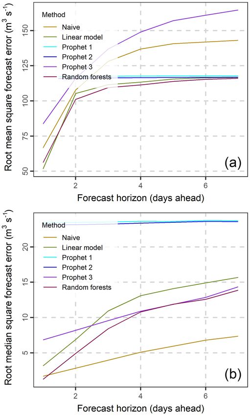
202G. A. Papacharalampous and H. Tyralis: Evaluation of random forests and Prophet for daily streamflow forecasting

Figure 1. Mean daily streamflow of Current river at Doniphan, Missouri (longitude: −90.85, latitude: 36.62) for the years 1981–2013.

Figure 2. Sample autocorrelation of the daily streamflow of the Current river and sample cross-correlation with the daily precipitation of the
basin. The sample cross-correlation is the estimate of Corr[xi , yi+j ], where Corr is the cross-correlation function.

and Papacharalampous et al. (2017a, 2018a, b). Prophet is                Addor et al. (2017b, see also the data availability section).
an automatic time series forecasting model, which also al-               The sample autocorrelation Corr[yi , yi+j ] and the sample
lows the incorporation of predictor variables, as well as                cross-correlation Corr[xi , yi+j ] are presented in Fig. 2. The
the computation of prediction intervals. The latter is pro-              sample autocorrelation is higher than 0.4 for time lag up to
posed, for instance, in Tyralis and Koutsoyiannis (2014). Pa-            three days, while the sample cross-correlation is higher than
pacharalampous et al. (2018c) investigate the performance of             0.4 for time lag up to two days. A correlation equal to 0.4
Prophet in monthly temperature and precipitation forecast-               means that the predictor variable can explain approximately
ing without utilizing predictor variables. This is also the way          16 % of the variance of the dependent variable in a linear re-
used herein. Since benchmarking forecasting results is es-               gression model between yi and xi .
sential, we implement a naïve method and a multiple linear                  Subsequently we present the forecasting methods of this
regression model alongside with the above outlined sophisti-             study, while further implementation details can be found
cated ones. Our aim is to illustrate important facts about the           in the code availability section. The forecasts of the naïve
models for the problem under examination.                                benchmark at time k + j , j = 1,. . . , 7 are equal to yk , i.e.
                                                                         they are equal to the last observation. The use of this
                                                                         benchmark is documented in Hyndman and Athanasopou-
2   Data and methods                                                     los (2018, Chap. 3.1). Multiple linear regression models are
                                                                         also widely implemented benchmarks (see Solomatine and
We forecast the mean daily streamflow of Current River at                Ostfeld, 2008). Herein, they are used for benchmarking the
Doniphan, Missouri (see Fig. 1). The daily precipitation data            results of random forests; therefore, the predictor variables
xi at the basin and the mean daily streamflow data yi span               utilized by these two methods are identical. These predictor
in the time period 1981–2013. This dataset was compiled by

Adv. Geosci., 45, 201–208, 2018                                                                       www.adv-geosci.net/45/201/2018/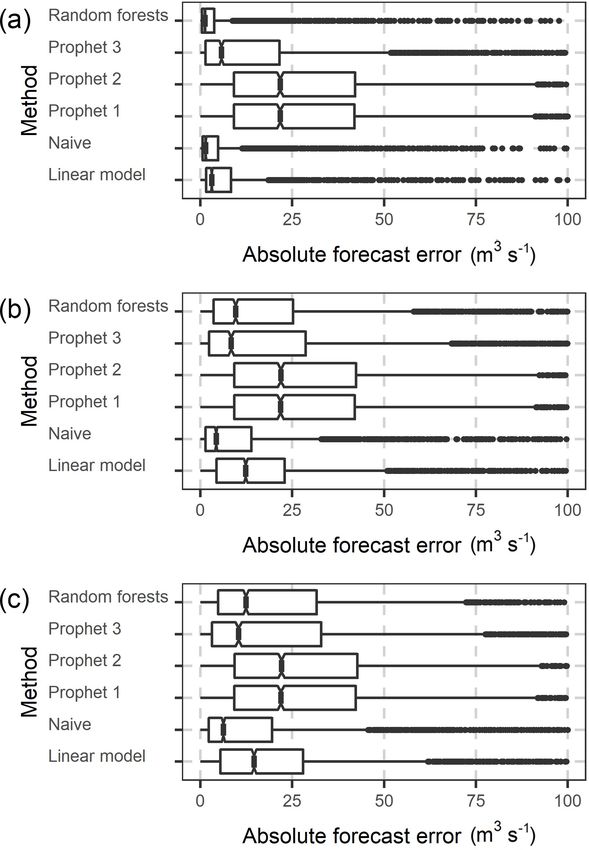
G. A. Papacharalampous and H. Tyralis: Evaluation of random forests and Prophet for daily streamflow forecasting203

Figure 3. 1-step ahead forecasts of the Current river daily streamflow in the periods 2004–2013 (a) and 2012–2013 (b).

variables are reported below together with the justification of        j = 1,. . . , 7. In this variation the seasonal component is au-
their selection. For the same methods, streamflow and pre-             tomatically handled by Prophet. Prophet 3 uses the last 30
cipitation data are pre-processed using the square root, as            observed values for fitting.
proposed by Messner (2018), with the aim for them to be                   Literature and technical information on the implementa-
normalized.                                                            tion of random forests is available in Verikas et al. (2011),
   Prophet is based on the idea of fitting Generalized Ad-             and Biau and Scornet (2016). Random forests are easy to
ditive Models. Its documentation is available in Taylor and            tune and implement due to the low number of parameters
Letham (2018a), while details about its software implemen-             (see also Scornet et al., 2015). Their main parameter is the
tation can be found in Taylor and Letham (2018b). We ex-               number of trees. Higher number of trees results in predictions
amine three variations of the Prophet model. In the first vari-        that are more accurate; however, in this case the computation
ation (hereafter named as “Prophet 1”; the remaining varia-            time increases substantially, while there is also an asymptotic
tions are named in a similar way) we decompose the stream-             limit in the accuracy of the model (see, for example, Biau
flow time series up to time k using the STL method (Cleve-             and Scornet, 2016). We use 100 trees, which is considered
land et al., 1990) and remove the seasonal component. Then             as a reasonable and balanced choice regarding their accu-
Prophet is fitted to the decomposed time series, it forecasts at       racy (with respect to the limit of accuracy) and computational
times k + j , j = 1,. . . , 7 and, finally, the seasonal component     cost (Probst and Boulesteix, 2018). The other parameters are
is added to the forecast. Prophet 2 is fitted to the stream-           set equal to the default values, as in the implementation by
flow time series up to time k, and forecasts at times k + j ,          Wright (2018). To forecast 1-step ahead (i.e. to forecast yk+1 )

www.adv-geosci.net/45/201/2018/                                                                      Adv. Geosci., 45, 201–208, 2018
204G. A. Papacharalampous and H. Tyralis: Evaluation of random forests and Prophet for daily streamflow forecasting
we use xk−2 , xk−1 , xk , yk−3 , yk−2 , yk−1 , yk and the month of
the yk+1 as predictor variables. We also used a lower num-
ber of predictor variables and the performance (not presented
here for reasons of brevity) was similar. Using more predic-
tor variables would result in considerably higher computa-
tion time with little expected gain in performance. We use
the month of yk+1 for considering the seasonality effect. To
forecast yk+2 we use again xk−2 , xk−1 , xk , yk−3 , yk−2 , yk−1 ,
yk and the month of yk+2 as predictor variables. We apply
the same procedure to forecast yk+j , j = 3,. . . , 7. Regard-
ing the training period, if we want to forecast yk+1 , random
forests are fitted using the respective xi−3 , xi−2 , xi−1 ,yi−4 ,
yi−3 , yi−2 , yi−1 as predictor variables and yi as dependent
variable for i = 1,. . . , k. Each time that a new forecast is re-
quired (i.e. when i increases by 1), the model is trained again,
so that it includes the latest information. A similar procedure
is followed for longer forecast horizons.
Forecasting is performed for all days in the years 2004–
2013. The reason for using 1/3 of the dataset for testing is
justified on the ground of the large variability of streamflow
explained from climatic and other factors (e.g. Kingston et
al., 2006; Li et al., 2018; Tyralis et al., 2018). Testing in an
independent set is also a standard practice in the assessment
of data-driven models (e.g. Solomatine and Ostfeld, 2008;
Elshorbagy et al., 2010a, b; Wu et al., 2014). In particular
for observations up to day k we forecast the streamflow at
days k + j , j = 1,. . . , 7. We produce forecasts for values of k
in {2003-12-21,. . . , 2013-12-30}. The forecasts are summa-
rized conditional upon the forecasting method and the fore-
cast horizon.
3 Results
Section 3 is devoted to the presentation of the results, which
Figure 4. Root mean square forecast errors (a) and root median
emphasizes on the 1-, 4- and 7-day ahead forecasts. In
square forecast errors (b).
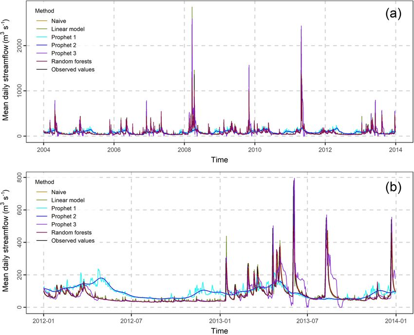
Figs. S1 and S2 (see the Supplement) we present these fore-
casts in comparison to the observations, while Fig. 3 focuses
on the 1-day ahead forecasts. The differences between the
methods are better presented in Fig. S2 in the Supplement.
This figure zooms in the period 2012–2013. In general, the for short forecast horizons (with length less than three days).
forecasts of the naïve, multiple linear regression and random For forecast horizons longer than four days random forests
forests methods are close to their target values. When the still perform the best, while Prophet 1 and 2 are better than
length of the forecast horizon increases, the distance between the naïve and Prophet 3 methods. The performance of the
the observations and the forecasts increases as well. The fore- naïve, multiple linear regression and random forests meth-
casts of Prophet 1 and 2 are smooth lines, i.e. they do not cap- ods decreases with increasing length of the forecast horizon
ture the abrupt streamflow changes. In addition, they lay far and gets stabilized for long forecast horizons due to the re-
from the actual streamflow values. The forecasts of Prophet 3 duction of the available information used by the predictor
seem to be in better agreement with the observed streamflow; variables. Prophet 1 and 2, on the other hand, seem to have
still, they are worse than those produced by the naïve, multi- a constant performance for all forecast horizons. In terms of
ple linear regression and random forests methods. RMdSE the naïve method is better than Prophet 3, which in
In Fig. 4 we present the root mean square errors (RMSE) turn is better than Prophet 1 and 2 for all forecast horizons.
and root median square errors (RMdSE) for all forecast hori- The performance of Prophet 1 and 2 is constant regardless of
zons. Random forests have the lowest RMSE followed by the the forecast horizon. Random forests are the best method for
multiple linear regression, the naïve and Prophet 3 methods the 1-day ahead forecast horizon, and the second best for the
Adv. Geosci., 45, 201–208, 2018 www.adv-geosci.net/45/201/2018/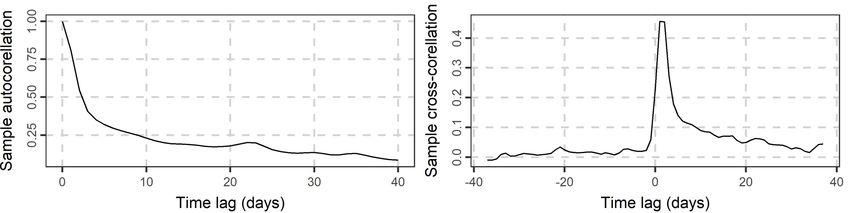
G. A. Papacharalampous and H. Tyralis: Evaluation of random forests and Prophet for daily streamflow forecasting205
Figure 5. Notched boxplots of the absolute forecast errors of the 1, 4
and 7-step ahead forecasts (a to c) of the daily streamflow of Current
river in the period 2004–2013. The x axis of the three graphs has
been truncated at 100 m3 s−1 .
2-day ahead and higher forecast horizons. RMdSE is lower
than RMSE for all methods.
To further investigate the above rankings and the differ-
ence in the magnitude between RMSE and RMdSE, in Fig. 5
we present the notched boxplots of the absolute errors for
the 1-, 4- and 7-day ahead forecast horizons. The medians of
the absolute error are similar to the RMdSE values presented
in Fig. 4. The boxplots are positively skewed, resulting in
higher RMSE than RMdSE values. In addition, the disper-
sion of absolute errors is higher for longer forecast horizons.
To understand how close the forecasts are to their corre-
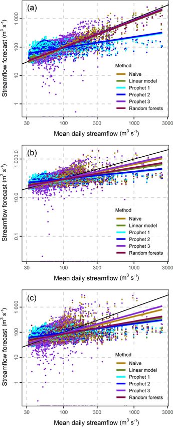
sponding observations we present the scatterplots of Fig. 6.
For all the methods excluding Prophet 1 and 2 the plots of
the linear models fitted between the forecasts and the ob-
Figure 6. 1-, 4- and 7-step ahead forecasts (a to c) and their corre-
servations are close to the black line, which corresponds to
sponding mean daily streamflow values. The black line corresponds
forecasts equal to the observations, indicating a good per-
to forecasts equal to observations, while the remaining lines are the
formance in 1-day ahead forecasting. The distance between plots of the linear regression models fitted between forecasts and
the black line and the other linear regression lines increases, observations.
www.adv-geosci.net/45/201/2018/ Adv. Geosci., 45, 201–208, 2018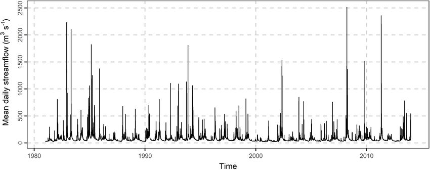
206G. A. Papacharalampous and H. Tyralis: Evaluation of random forests and Prophet for daily streamflow forecasting

when the forecast horizon increases. The increase is less pro-        Data availability. The data used in the present study can be ob-
nounced for the Prophet 1 and 2 methods.                              tained from the CAMELS dataset (Addor et al., 2017a, b; New-
                                                                      man et al., 2014, 2015). The daily precipitation data included in the
                                                                      CAMELS dataset were sourced by Thornton et al. (2014).
4   Discussion and conclusions

In summary, the following remarks are important, especially           Supplement. The supplement related to this article is available
in light of Abrahart et al. (2008) who comment on the need            online at: https://doi.org/10.5194/adgeo-45-201-2018-supplement.
for documenting the performance assessment of data-driven
models on the grounds of specific questions. Random forests
                                                                      Competing interests. The authors declare that they have no conflict
are a better predictor compared to the multiple linear re-
                                                                      of interest.
gression models, while they outperform the naïve method
in terms of root mean square error. The use of the selected
precipitation predictor variables considerably improves the           Acknowledgements. We thank the Editor Luke Griffiths and one
forecasts, probably due to the nature of the examined prob-           anonymous reviewer, whose comments have led to the improve-
lem; however, their influence diminishes for forecast hori-           ment of this paper.
zons longer than four days. This is also expected from the
magnitude of autocorrelations and cross-correlations with             Edited by: Luke Griffiths
precipitation, which indicate that precipitation should influ-        Reviewed by: Luke Griffiths and one anonymous referee
ence the magnitude of streamflow for some days. The fore-
casting error of the Prophet 1 and 2 methods (which are fitted
to the whole sample) is independent of the forecast horizon.          References
Nevertheless, these two methods perform consistently worse
than the other methods in terms of root median square error,          Abrahart, R. J., See, L. M., and Dawson, C. W.: Neural Network
while they have a comparable (to the other methods) per-                 Hydroinformatics: Maintaining Scientific Rigour, in: Practical
formance in terms of root mean square error. Furthermore,                Hydroinformatics, edited by: Abrahart, R. J., See, L. M., and
Prophet exhibits a worse performance than the naïve method               Solomatine, D. P., Springer-Verlag Berlin Heidelberg, 33–47,
                                                                         https://doi.org/10.1007/978-3-540-79881-1_3, 2008.
when it exclusively uses observations from the last 30 days
                                                                      Addor, N., Newman, A. J., Mizukami, N., and Clark, M. P.:
(Prophet 3). Random forests are a good method for obtaining
                                                                         Catchment attributes for large-sample studies, Boulder, CO,
optimal forecasts, while their performance could be further              UCAR/NCAR, https://doi.org/10.5065/D6G73C3Q, 2017a.
improved by using more predictor variables, e.g. temperature          Addor, N., Newman, A. J., Mizukami, N., and Clark, M. P.: The
variables. The naïve method is also good; therefore, it should           CAMELS data set: catchment attributes and meteorology for
be used as a benchmark, in spite of the fact that it is rarely           large-sample studies, Hydrol. Earth Syst. Sci., 21, 5293–5313,
met in the hydrological forecasting literature. The Prophet              https://doi.org/10.5194/hess-21-5293-2017, 2017b.
model should be used for forecasting at long horizons.                Allaire, J. J., Xie, Y., McPherson, J., Luraschi, J., Ushey, K.,
   We note that this study is among the first implementing               Atkins, A., Wickham, H., Cheng, J., and Chang, W.: rmark-
random forests and Prophet for streamflow forecasting. We                down: Dynamic Documents for R. R package version 1.10, avail-
have thoroughly investigated the performance of all meth-                able at: https://CRAN.R-project.org/package=rmarkdown (last
                                                                         access: 16 August 2018), 2018.
ods, looking at their predictive performance at several fore-
                                                                      Auguie, B.: gridExtra: Miscellaneous Functions for “Grid” Graph-
cast horizons. The visualization of all aspects helped in bet-
                                                                         ics, R package version 2.3, available at: https://CRAN.R-project.
ter understanding important facts about the models’ perfor-              org/package=gridExtra (last access: 16 August 2018), 2017.
mance and, thus, could be used as a guide for the assessment          Biau, G. and Scornet, E.: A random forest guided tour, TEST, 25,
of methods in streamflow forecasting.                                    197–227, https://doi.org/10.1007/s11749-016-0481-7, 2016.
                                                                      Breiman, L.: Random Forests, Mach. Learn., 45, 5–32,
                                                                         https://doi.org/10.1023/A:1010933404324, 2001.
Code availability. This paper is easily reproducible using the R      Cleveland, R. B., Cleveland, W. S., McRae, J. E., and Terpenning,
Programming Language (R Core Team, 2018). We used the follow-            I.: STL: A Seasonal-Trend Decomposition Procedure Based on
ing R packages: bestNormalize (Peterson, 2018), devtools (Wick-          Loess, J. Off. Stat., 6, 3–33, 1990.
ham et al., 2018b), gdata (Warnes et al., 2017), ggplot2 (Wickham,    Elshorbagy, A., Corzo, G., Srinivasulu, S., and Solomatine, D.
2016; Wickham et al., 2018a), gridExtra (Auguie, 2017), knitr (Xie,      P.: Experimental investigation of the predictive capabilities of
2014; 2015; 2018), lubridate (Grolemund and Wickham, 2011;               data driven modeling techniques in hydrology – Part 1: Con-
Spinu et al., 2018), prophet (Taylor and Letham, 2018b), ranger          cepts and methodology, Hydrol. Earth Syst. Sci., 14, 1931–1941,
(Wright, 2018; Wright and Ziegler, 2017), readr (Wickham et al.,         https://doi.org/10.5194/hess-14-1931-2010, 2010a.
2017), rmarkdown (Allaire et al., 2018), scales (Wickham, 2018),      Elshorbagy, A., Corzo, G., Srinivasulu, S., and Solomatine,
stringi (Gagolewski, 2018), zoo (Zeileis and Grothendieck, 2005;         D. P.: Experimental investigation of the predictive capabil-
Zeileis et al., 2018).                                                   ities of data driven modeling techniques in hydrology –

Adv. Geosci., 45, 201–208, 2018                                                                    www.adv-geosci.net/45/201/2018/
G. A. Papacharalampous and H. Tyralis: Evaluation of random forests and Prophet for daily streamflow forecasting207
Part 2: Application, Hydrol. Earth Syst. Sci., 14, 1943–1961, within a purely statistical framework, Geosci. Lett., 5,
https://doi.org/10.5194/hess-14-1943-2010, 2010b. https://doi.org/10.1186/s40562-018-0111-1, 2018b.
Gagolewski, M.: stringi: Character String Processing Facilities, R Papacharalampous, G., Tyralis, H., and Koutsoyiannis, D.: Pre-
package version 1.2.4, available at: https://CRAN.R-project.org/ dictability of monthly temperature and precipitation using auto-
package=stringi (last access: 16 August 2018), 2018. matic time series forecasting methods, Acta Geophys., 66, 807–
Grolemund, G. and Wickham, H.: Dates and Times 831, https://doi.org/10.1007/s11600-018-0120-7, 2018c.
Made Easy with lubridate, J. Stat. Softw., 40, Peterson, R. A.: bestNormalize: Normalizing Transformation Func-
https://doi.org/10.18637/jss.v040.i03, 2011. tions, R package version 1.2.0, available at: https://CRAN.
Hyndman, R. J. and Athanasopoulos, G.: Forecasting: Principles R-project.org/package=bestNormalize (last access: 16 August
and Practice, available at: https://otexts.org/fpp2/ (last access: 16 2018), 2018.
August 2018), 2018. Petty, T. R. and Dhingra, P.: Streamflow Hydrology Estimate Using
Jain, S. K., Mani, P., Jain, S. K., Prakash, P., Singh, V. P., Tullos, D., Machine Learning (SHEM), J. Am. Water Resour. As., 54, 55–
Kumar, S., Agarwal, S. P., and Dimri, A. P.: A Brief review of 68, https://doi.org/10.1111/1752-1688.12555, 2018.
flood forecasting techniques and their applications, Int. J. River Probst, P. and Boulesteix, A. L.: To tune or not to tune the number
Basin Man., https://doi.org/10.1080/15715124.2017.1411920, of trees in random forest, J. Mach. Learn. Res., 18, 1–18, 2018.
2018. R Core Team: R: A language and environment for statistical com-
Kingston, D. G., Lawler D. M., and McGregor, G. R.: Linkages puting, R Foundation for Statistical Computing, Vienna, Austria,
between atmospheric circulation, climate and streamflow in the available at: https://www.R-project.org/ (last access: 16 August
northern North Atlantic: research prospects, Prog. Phys. Geogra- 2018), 2018.
phy, 30, 143–174, https://doi.org/10.1191/0309133306pp471ra, Scornet, E., Biau, G., and Vert, J. P.: Consistency of random forests,
2006. Ann. Stat., 43, 1716–1741, https://doi.org/10.1214/15-AOS1321,
Li, L., Schmitt, R. W., and Ummenhofe, C. C.: The role of 2015.
the subtropical North Atlantic water cycle in recent US ex- Shortridge, J. E., Guikema, S. D., and Zaitchik, B. F.: Machine
treme precipitation events, Clim. Dynam., 50, 1291–1305, learning methods for empirical streamflow simulation: a com-
https://doi.org/10.1007/s00382-017-3685-y, 2018. parison of model accuracy, interpretability, and uncertainty in
Lima, A. R., Cannon, A. J., and Hsieh, W. W.: Nonlinear regression seasonal watersheds, Hydrol. Earth Syst. Sci., 20, 2611–2628,
in environmental sciences using extreme learning machines: A https://doi.org/10.5194/hess-20-2611-2016, 2016.
comparative evaluation, Environ. Model. Softw., 73, 175–188, Solomatine, D. P. and Ostfeld, A.: Data-driven modelling: some
https://doi.org/10.1016/j.envsoft.2015.08.002, 2015. past experiences and new approaches, J. Hydroinform., 10, 3–
Messner, J. W.: Chapter 11 – Ensemble Postprocessing With R, in: 22, https://doi.org/10.2166/hydro.2008.015, 2008.
Statistical Postprocessing of Ensemble Forecasts, edited by: Van- Spinu, V., Grolemund, G., and Wickham, H.: lubridate: Make Deal-
nitsem, S., Wilks, D. S., and Messner, J. W., Elsevier, 291–329, ing with Dates a Little Easier, R package version 1.7.4, avail-
https://doi.org/10.1016/B978-0-12-812372-0.00011-X, 2018. able at: https://CRAN.R-project.org/package=lubridate (last ac-
Newman, A. J., Sampson, K., Clark, M. P., Bock, A., Viger, R. cess: 16 August 2018), 2018.
J., and Blodgett, D.: A large-sample watershed-scale hydrom- Taylor, S. J. and Letham, B.: Forecasting at scale, Am. Stat., 72,
eteorological dataset for the contiguous USA, Boulder, CO, 37–45, https://doi.org/10.1080/00031305.2017.1380080, 2018a.
UCAR/NCAR, https://doi.org/10.5065/D6MW2F4D, 2014. Taylor, S. J. and Letham, B.: prophet: Automatic Forecasting Pro-
Newman, A. J., Clark, M. P., Sampson, K., Wood, A., Hay, L. cedure, R package version 0.3.0.1, available at: https://CRAN.
E., Bock, A., Viger, R. J., Blodgett, D., Brekke, L., Arnold, J. R-project.org/package=prophet (last access: 16 August 2018),
R., Hopson, T., and Duan, Q.: Development of a large-sample 2018b.
watershed-scale hydrometeorological data set for the contiguous Thornton, P. E., Thornton, M. M., Mayer, B. W., Wilhelmi,
USA: data set characteristics and assessment of regional variabil- N., Wei, Y., Devarakonda, R., and Cook, R. B.: Daymet:
ity in hydrologic model performance, Hydrol. Earth Syst. Sci., Daily Surface Weather Data on a 1-km Grid for North Amer-
19, 209–223, https://doi.org/10.5194/hess-19-209-2015, 2015. ica, Version 2, ORNL DAAC, Oak Ridge, Tennessee, USA,
Papacharalampous, G., Tyralis, H., and Koutsoyiannis, D.: Er- https://doi.org/10.3334/ORNLDAAC/1219, 2014.
ror evolution in multi-step ahead streamflow forecasting for Tyralis, H. and Koutsoyiannis, D.: A Bayesian statistical model for
the operation of hydropower reservoirs, Preprints, 2017100129, deriving the predictive distribution of hydroclimatic variables,
https://doi.org/10.20944/preprints201710.0129.v1, 2017a. Clim. Dynam., 42, 2867–2883, https://doi.org/10.1007/s00382-
Papacharalampous, G., Tyralis, H., and Koutsoyiannis, D.: Fore- 013-1804-y, 2014.
casting of geophysical processes using stochastic and machine Tyralis, H. and Papacharalampous, G.: Variable selection in
learning algorithms, Eur. Water, 59, 161–168, 2017b. time series forecasting using random forests, Algorithms, 10,
Papacharalampous, G., Tyralis, H., and Koutsoyiannis, D.: Com- https://doi.org/10.3390/a10040114, 2017.
parison of stochastic and machine learning methods for multi- Tyralis, H. and Papacharalampous, G. A.: Large-scale assessment
step ahead forecasting of hydrological processes, Preprints, of Prophet for multi-step ahead forecasting of monthly stream-
2017100133, https://doi.org/10.20944/preprints201710.0133.v2, flow, Adv. Geosci., 45, 147–153, https://doi.org/10.5194/adgeo-
2018a. 45-147-2018, 2018.
Papacharalampous, G., Tyralis, H., and Koutsoyiannis, D.: Tyralis, H., Dimitriadis, P., Koutsoyiannis, D., O’Connell, P. E.,
One-step ahead forecasting of geophysical processes Tzouka, K., and Iliopoulou, T.: On the long-range dependence
properties of annual precipitation using a global network of in-
www.adv-geosci.net/45/201/2018/ Adv. Geosci., 45, 201–208, 2018208G. A. Papacharalampous and H. Tyralis: Evaluation of random forests and Prophet for daily streamflow forecasting
strumental measurements, Adv. Water Resour., 111, 301–318, Wright, M. N.: ranger: A Fast Implementation of Random Forests,
https://doi.org/10.1016/j.advwatres.2017.11.010, 2018. R package version 0.10.1, available at: https://CRAN.R-project.
Verikas, A., Gelzinis, A., and Bacauskiene, M.: Min- org/package=ranger (last access: 16 August 2018), 2018
ing data with random forests: A survey and re- Wright, M. N. and Ziegler, A.: ranger: A Fast Implementation of
sults of new tests, Pattern Recogn., 44, 330–349, Random Forests for High Dimensional Data in C++ and R, J.
https://doi.org/10.1016/j.patcog.2010.08.011, 2011. Stat. Softw., 77, https://doi.org/10.18637/jss.v077.i01, 2017.
Warnes, G. R., Bolker, B., Gorjanc, G., Grothendieck, G., Korosec, Wu, W., Dandy, G. C., and Maier, H. R.: Protocol for develop-
A., Lumley, T., MacQueen, D., Magnusson, A., and Rogers, J.: ing ANN models and its application to the assessment of the
gdata: Various R Programming Tools for Data Manipulation, quality of the ANN model development process in drinking wa-
R package version 2.18.0, available at: https://CRAN.R-project. ter quality modelling, Environ. Modell. Softw., 54, 108–127,
org/package=gdata (last access: 16 August 2018), 2017. https://doi.org/10.1016/j.envsoft.2013.12.016, 2014.
Wickham, H.: ggplot2, Springer International Publishing, Xie, Y.: knitr: A Comprehensive Tool for Reproducible Research
https://doi.org/10.1007/978-3-319-24277-4, 2016. in R, in: Implementing Reproducible Computational Research,
Wickham, H.: scales: Scale Functions for Visualization, R pack- Chapman and Hall/CRC, 2014.
age version 1.0.0, available at: https://CRAN.R-project.org/ Xie, Y.: Dynamic Documents with R and knitr, 2nd edition, Chap-
package=scales (last access: 16 August 2018), 2018. man and Hall/CRC, 2015.
Wickham, H., Hester, J., and Francois, R.: readr: Read Rectan- Xie, Y.: knitr: A General-Purpose Package for Dynamic Report
gular Text Data, R package version 1.1.1, available at: https: Generation in R, R package version 1.20, available at: https:
//CRAN.R-project.org/package=readr (last access: 16 August //CRAN.R-project.org/package=knitr (last access: 16 August
2018), 2017. 2018), 2018.
Wickham, H, Chang, W., Henry, L., Pedersen, T. L., Takahashi, K., Zeileis, A. and Grothendieck, G.: zoo: S3 infrastructure
Wilke, C., and Woo, K.: ggplot2: Create Elegant Data Visualisa- for regular and irregular time series, J. Stat. Softw., 14,
tions Using the Grammar of Graphics, R package version 3.0.0, https://doi.org/10.18637/jss.v014.i06, 2005.
available at: https://CRAN.R-project.org/package=ggplot2 (last Zeileis, A., Grothendieck, G., and Ryan, J. A.: zoo: S3 Infrastruc-
access: 16 August 2018), 2018a. ture for Regular and Irregular Time Series (Z’s Ordered Obser-
Wickham, H., Hester, J., and Chang, W.: devtools: Tools to Make vations), R package version 1.8-3, available at: https://CRAN.
Developing R Packages Easier, R package version 1.13.6, avail- R-project.org/package=zoo (last access: 16 August 2018), 2018.
able at: https://CRAN.R-project.org/package=devtools (last ac- Zhang, Z., Zhang, Q., and Singh, V. P.: Univariate streamflow
cess: 16 August 2018), 2018b. forecasting using commonly used data-driven models: litera-
ture review and case study, Hydrolog. Sci. J., 63, 1091–1111,
https://doi.org/10.1080/02626667.2018.1469756, 2018.
Adv. Geosci., 45, 201–208, 2018 www.adv-geosci.net/45/201/2018/You can also read