Large Scale Sign Detection using HOG Feature Variants
←
→
Page content transcription
If your browser does not render page correctly, please read the page content below
Large Scale Sign Detection using HOG Feature Variants
Gary Overett and Lars Petersson
NICTA, Locked Bag 8001, Canberra, Australia
{gary.overett,lars.petersson}@nicta.com.au
Abstract— In this paper we present two variant formulations positive rates (< 10−9 ) for many sign detection problems,
of the well-known Histogram of Oriented Gradients (HOG) the large volume of data we are processing in tandem with
features and provide a comparison of these features on a large the extreme sparsity of traffic signs within a road scene
scale sign detection problem. The aim of this research is to
find features capable of driving further improvements atop a mean that we still have need of more powerful features
preexisting detection framework used commercially to detect able to further reduce false positive rates when our currently
traffic signs on the scale of entire national road networks (1000’s available features are no longer able to.
of kilometres of video). We assume the computationally efficient
If we accept that more powerful and complex features will
framework of a cascade of boosted weak classifiers. Rather than
comparing features on the general problem of detection we generally be more computationally intensive [2] we must also
compare their merits in the final stages of a cascaded detection accept that they may not be suitable for the entire evaluation
problem where a feature’s ability to reduce error is valued more chain of a classifier. However, if we maintain our use of fast-
highly than computational efficiency. to-evaluate features at the head of a detection cascade and
Results show the benefit of the two new features on a
use more powerful and more complex features at the tail end
New Zealand speed sign detection problem. We also note the
importance of using non-sign training and validation instances of a cascade we are able to maintain fast average evaluation
taken from the same video data that contains the training and times. By using these powerful features only to resolve the
validation positives. This is attributed to the potential for the class/non-class status of a tiny minority (see Figure 1) of the
more powerful HOG features to overfit on specific local patterns input imagery we are able to benefit from their discriminative
which may be present in alternative video data.
power at negligible computational time cost.
I. INTRODUCTION
Automatic traffic sign detection is an important problem
for driver assistance systems and automatic mapping applica-
tions. In this paper we aim to improve upon a preexisting sign
detection framework used commercially in large scale1 map-
ping applications. A key challenge in this work is producing
classifiers which are able to scan large video datasets quickly,
while achieving high detection rates2 (≈ 99%) and minimal
false positive rates (≈ 10−9 ) despite the huge volume of
input image data and the relative sparsity of traffic signs
within a typical road scene.
The authors of this paper have previously promoted [1],
[2] a viewpoint that both error rates and time to decision
determine the value of a given detection solution. This re-
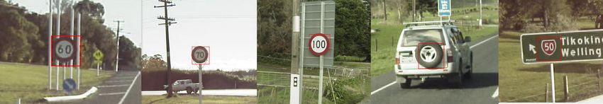
search has contributed to the development of a highly robust Fig. 1. New Zealand speed signs (top three rows) and challenging speed
traffic sign detection platform used commercially on 1000’s sign false positives (bottom three rows). The speed sign false positives
shown here represent a tiny minority (5 × 10⁻¹⁰ of windows scanned)
of kilometres of on road video. This includes the histogram of non speed signs remaining after a four stage classifier. Logos, wheels
feature [1] and the LiteHOG+ feature [2] which are both and other signs make up a large portion of difficult false positives. These
extremely computationally efficient, even when compared challenging instances require more powerful features to further reduce the
error rate of the classifier.
to other efficient features such as Haar features [3]. While
the Histogram and LiteHOG+ features can achieve excellent
detection rates in combination with extremely low false This paper is organised as follows: Initially we present
some background information covering prior work. This is
1 Results shown in this paper consider a video dataset of 15 million followed by an explanation of our baseline sign detection
1024×768 image frames taken at 10 meter intervals from a vehicle mounted framework. Next we outline two previously unpublished
camera system deployed in New Zealand. Histogram of Oriented Gradient based features which are
2 All false positive rates indicated in this paper are calculated per-
used to extend the baseline system to further reduce the
classifier-inspected-window. A typical single frame of video may be in-
spected more than a million times as the detector is run over multiple scales detector false positive rate. Finally we include an analysis
and locations in the frame. of the results using speed sign training and validation tasks.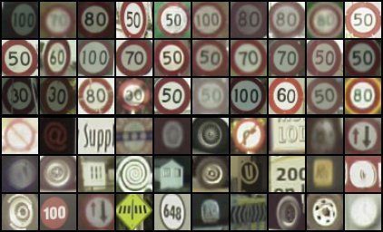
II. BACKGROUND                                     A short cascade structure: While several other detectors
                                                                      found in literature have used a cascade detector structure [3],
   Given the importance of sign detection in several appli-
                                                                      [11], [12], [13] all of these have tended to consist of a large
cations there is a significant amount of previous literature
                                                                      number of cascade stages (more than 20 in [12] and [13]).
dedicated to the subject [4], [5], [6], [7], [8], [9]. Unfortu-
                                                                      In contrast, we employ a short cascade with just five stages.
nately, very little of this research deals with high volumes
                                                                      Since each stage will likely reduce the detection rate, many
of video data exposed to real world problems.
                                                                      stages can become a liability to the maintenance of a high
   Many previous sign detectors have employed the use of
                                                                      detection rate. Even if very ambitious per stage detection
color sensitive features to take advantage of the strong color
                                                                      rates are specified these must be set against a validation
cues used in traffic signs [4], [5], [8]. Broggi et al. [8] present
                                                                      population which may not be a reliable indicator of the actual
a real time road sign detector using color segmentation,
                                                                      detection rate which will be a achieved.
shape recognition and neural network learning. Lafuente-
                                                                         The LogitBoost [14] Learning Algorithm: The time-
Arroyo et al. [4] employ color and shape information within
                                                                      constrained nature of our final application means that we
a Support Vector Machine (SVM) based classifier. Bahlmann
                                                                      require a learning algorithm providing efficient classifiers,
et al. [5] apply a standard Haar feature based approach to
                                                                      boosting meets this criteria. Of the large number of boosting
independent color channel information. Paulo and Correia
                                                                      algorithms available [14], [15], [16] we have selected
[6] have used red and blue color information as an initial
                                                                      LogitBoost [14] as our chosen approach. The motivation for
cue for a sign detection system. Signs are then further
                                                                      this is that we have found it to be the most consistently
classified using shape information into several broad sub-
                                                                      superior on a sign detection task when compared to others
categories such as ‘danger’ and ‘information’. While the
                                                                      we have considered (Including AdaBoost, RealBoost [15]
approach and features adopted in our research have been
                                                                      and GentleBoost [14]).
applied to color information [10] we will limit the scope of
                                                                         LiteHOG+ [2] as the Default Feature: Again the time-
our experimental results in this paper to those obtained using
                                                                      constrained nature of our application means that we cannot
grayscale imagery in order to maintain a simpler platform for
                                                                      move away from an extremely fast feature such as LiteHOG+
comparisons.
                                                                      for the majority of the cascade evaluation work.
   Alefs et al. [7] present a road sign detection framework
                                                                         Speed Signs as the Object Class: This paper makes no
using edge orientation histograms as the main feature. More
                                                                      specific sign type assumptions although we have chosen to
recently, Timofte et al. [9] detailed a full sign detection
                                                                      use the New Zealand speed sign as a test case. Of the many
algorithm employing Haar-like features which automatically
                                                                      traffic sign types we consider to be of interest, speed signs
acquires a 3D localisation (geo-location) of the detected
                                                                      are among the most abundant within a typical road scene.
signs. While this method does commit to some sign specific
                                                                      By dividing our New Zealand video according to the natural
shape based techniques it is shown to produce excellent
                                                                      geographic division between the country’s north and south
results across a range of sign types and circumstances.
                                                                      islands we get a training population of 57377 speed signs
   A major distinguishing feature of this research from prior
                                                                      from the north island with a validation population of 21500
work by others is the use of large scale training and vali-
                                                                      signs from the south island. By merging all speed signs into
dation real world video data (see Figure 1). This enables us
                                                                      a single sign type we create a sign class which is relatively
to perform a direct performance comparison of alternative
                                                                      challenging, since a general speed sign detector must capture
detectors at the scale in which the system will be deployed,
                                                                      the properties of a variety of face values in a single detector.
on video of entire national road networks. Training and
validation is performed using a 15 million 1024×768 image                      IV. P REVIOUS HOG I MPLEMENTATIONS
frames collected at a geospatial frequency of 10 meters                  In the literature, the name “Histograms of Oriented Gra-
across New Zealand. To our knowledge this is the largest              dients” or HOG has been used to refer to a number of
validation task ever presented for a sign detection problem.          unique but related features. Differences vary in terms of the
                                                                      shape and size of the local region over which a histogram
           III. A BASELINE D ETECTION S YSTEM
                                                                      may be calculated, the range of orientations allocated to
   In this section we introduce our baseline experimental             a single histogram bin, the normalisations (if any) applied
detector against which we can test our two prospective HOG            to the gradients, and the manner in which the descriptor
features. Since the construction and design of this preexisting       responses are combined by a machine learning method or
detector differs somewhat to that found in prior literature its       other approach.
implementation warrants both description and justification.              The power of HOG features came to prominence via
   The aim of our detector creation process is ideally to yield       the work of Dalal and Triggs [17] who demonstrated its
a three to five stage classifier. The final classifier should aim     superiority above a number of features in a basic pedestrian
to achieve a 99% detection rate with a false positive rate            detection problem. This original work provided a plethora of
below 10−9 . Some applications require false positive rates           closely related HOG variants which it compared on its own
as low as 10−11 to 10−12 .                                            INRIA pedestrian dataset. The authors follow the approach
   The following elements are used in the creation of our             of varying a number of parameters in order to find some
baseline detector:                                                    degree of “optimal” HOG feature. Notably, they compare
both rectangular and circular “cells” over which to sum where O ∈ {0, 1, . . . , 7} defines the orientation according to
gradients, and compare the merits of increasing the number Figure 2, R defines the set of points within a given rectan-
of orientation bins. At the learning level they apply Linear gular region, and GO () provides the L1 gradient magnitude
SVM learning to construct the final pedestrian detector. at coordinates (i, j) in the input image x.
Despite its successes on a challenging pedestrian detection
y
problem the evaluation of the Dalal and Triggs SVM classi- 3 1
fier is quite slow. In response Zhu et al. [11] created a much
faster HOG based pedestrian detector using an AdaBoost 2 0
x
trained classifier. The resulting HOG classifier yielded a
greater than 60 times speedup with comparable detection 6 4
performance. Two key differences in the work of Zhu et al. 7 5
as compared to the original Dalal and Triggs implementation
is the use of HOG features at a wide variety of scales and the Fig. 2. The orientation space is divided into 8 bins. Each pixel in the gray
image is assigned to one of these orientations.
per-histogram linearisation using individually trained SVM
classifiers for each feature.
In similar fashion to Zhu et al. we employ the use of
Our previously published feature, LiteHOG+ [2], is an
the integral image representation [3], [21] to optimise the
even more computationally efficient HOG feature. Limiting
summing of gradient magnitudes over various rectangular
the cell size over which gradients are summed to a 4 × 4
shapes R. Figure 3 shows the basic flow of computation
image region, greatly reduces the computational complexity
from the input image to the creation of the integral images.
of the feature.
The two HOG features presented in this paper are most
single orientation
closely aligned to those presented in [11] in that histograms Greyscale x and y
magnitude
&
integral image
image gradients
are taken over multiple shapes and scales and are combined orientation
using a boosting approach. Primarily what makes our two
features distinct from those of Zhu et al. is the manner in
which we create a linear class/non-class weak hypothesis Fig. 3. Computing the Histogram Integral Images. Given a grayscale image,
from the histogram response. the horizontal (x) and vertical (y) gradients of an image are computed at
every pixel using a [−1, 0, 1] kernel. This is then used to compute an L1
magnitude and discretised orientation for each pixel. The magnitude values
V. F ORMULATING N EW HOG F EATURE VARIANTS are subsequently separated according to 8 orientations (see Figure 2) which
are used to create 8 separate integral images.
As an ensemble method [18], boosting acts on a popula-
tion of weak hypotheses or models rather than the feature Given a positive and negative class population of scalar
responses themselves. Where Zhu et al. employ the use of feature responses f () we then train a weak hypothesis using
SVM to create the weak hypotheses we chose to use the the SRB learner. The trained S-HOG features can then be
Smoothed Response Binning (SRB) learner as used in [2], used in any ensemble learning algorithm. The performance
[19], [20]. An advantage of the SRB learner is its ability of S-HOG features is given in Section VI.
to learn multi modal distributions with high accuracy and a
low degree of overfitting when training populations are small. B. FDA Linearised HOG Feature (FDA-HOG)
However, no direct comparison has been made between SRB The second HOG feature we will deal with in this paper
learners and SVM applied as a weak learner. is the Fishers Discriminant Analysis (FDA) linearised HOG
feature (FDA-HOG). The idea here is to replace the SVM
A. Single Bin HOG Feature (S-HOG) learner used by Zhu et al. [11] with a linearisation obtained
using Fishers Discriminant Analysis [22]. This scalar re-
Rather than applying any form of SVM linearisation, sin- sponse can then be combined with an SRB learner as in
gle bin HOG features are constructed by taking the individual the S-HOG feature. The motivation for this is simple, FDA
histogram bins separately. By pairing the one dimensional S- can supply a linearisation in less time than it would take
HOG feature responses with an SRB learner we create the to train a local SVM classifier for each prospective feature.
weak hypotheses required by boosting. Furthermore, the evaluation of the final feature response is
Therefore the S-HOG feature response is calculated by simpler than evaluating an SVM classifier at run-time.
simply taking the sum of gradient magnitudes (aligned to As with the S-HOG feature we use 8 orientation bins
a single orientation bin) within a rectangular area to be as shown in Figure 2 and use L1 gradient magnitudes. In
the feature response. Equation 1 shows the formula for order to maximise the potential of the featurespace we allow
calculating the feature response f (x) of a single S-HOG masking of the 8 dimensional histograms to allow FDA to
feature. work on subsets of N histogram bins. We find the projection
X w using the canonical variate of FDA [22] via Equation 2.
f (O, R, x) = GO (i, j) (1)
−1
∀(i,j)∈R w = Sw (m1 − m2 ) (2)where w is the N dimensional projection matrix, Sw is instances we must also perform a manual ‘cleaning’ step
the within class scatter matrix and m1 , m2 are the means of to ensure that the negative training and test images are free
the positive and negative classes respectively. from actual speed signs.
This gives us the feature response:
TABLE II
P ER -S TAGE BASELINE C LASSIFIER I NFORMATION
f (Ō, R, x) = w · Φ(Ō, R, x) (3)
Stage # 1 2 3 4 5
where Ō is a vector containing the selected orientations # Features 35 200 400 600 1000
from {0, 1, . . . , 7}, R defines the set of points within a given # Feature Pool 4300 2048 2048 2048 2048
rectangular region, and Φ() supplies the histogram vector for Per-Stage False Neg. 0.02% 0.58% 0.24% 0.24% 0.24%
the gradient magnitudes within rectangle R in image x for Accum. Hit Rate 99.98% 99.40% 99.16% 98.92% 98.68%
the required orientations Ō. Per-Stage False Pos. 0.1% 0.1% 1% 5% 20%
Accum. False Pos 10−3 10−6 10−8 5×10⁻¹⁰ 10−10
As with the S-HOG feature the weak hypothesis is cal-
culated using the SRB learners trained with a population of
positive and negative training data. Table II shows the per stage training parameters. The
number of features in each stage is gradually increased with
VI. E XPERIMENTAL E VALUATION just 35 features in the initial stage. Essentially this is in
In accordance with our aim of finding more powerful accordance with a tried and tested formula used in many
features to improve our classifier performance at the tail of our other classifiers. The feature pool in Table II refers to
end of the detection problem we trained a baseline five the number of LiteHOG+ features which are made available
stage LiteHOG+ classifier using LogitBoost (see Section III). for selection in each training iteration during boosting. This
Tables I and II provide some detailed information about this feature pool is replaced with a random subset of the total
preexisting cascade. featurespace at each iteration, increasing the total number
of features available to the classifier. Experimentation shows
TABLE I that no improvements are made to classifier performance if
BASELINE C LASSIFIER I NFORMATION the feature pool is increased.
The accumulated false positive rate shown in Table II is
Sign Type New Zealand Speed Signs
calculated using the NICTA Road Scene DataBase (NICTA
# Training Positives 57377
# Validation Positives 21500
RSDB). This statistic is known to vary significantly between
# Training Negatives 160K videos from different scenes.
# Validation Negatives 40K In our first pair of experiments we replace the fifth stage
Negative Source NICTA Road Scene DataBase LiteHOG+ classifier with either an S-HOG or FDA-HOG
classifier, maintaining all other experimental parameters as
With regard to the training and validation positives shown shown in Tables I and II. In order to compare the fifth stage
in Table I we note that not all positive instances will pass LiteHOG+ feature with the S-HOG and FDA-HOG classifier
through to the later stages of the cascade since they will be we produce ROC (Receiver Operating Characteristic) curves
lost in the earlier stages in accordance with the false negative for each of the three classifiers. Rather than producing an
rates shown in Table II. Conversely, the number of training ROC curve for the entire range of false positive rates and hit
negatives supplied in each training iteration is held constant rates we limit our calculation to those values achievable given
by bootstrapping negative examples from the NICTA Road the preexisting four stages. This ‘locked in’ false negative
Scene DataBase (NICTA RSDB). This database includes a rate is indicated by the gray region of the ROC plot shown
collection of road scene videos collected in a diverse range in Figure 4.
of settings around the world, including numerous locations A. Native vs. Introduced Negatives
in Australia, the United States, Europe and China. The total
Statistical machine learning algorithms tend to learn pat-
amount of data which can be scanned for negatives includes
terns in training data which can be considered to be of two
over 10 Million video frames, primarily with a resolution
different categories, general patterns and specific patterns.
of 960 × 540. Bootstrapping from this database proceeds
General patterns are those that are represented in the training
for each stage with a calibration step aimed at calculating
data which can be said to describe an actual property in that
the sparsest sampling pattern which will yield sufficient
class of data in the real world. Specific patterns are those
samples to make up the negative training set. That is, for the
patterns which are present in the training data but may not
initial stages where false positive rates are still significant,
occur to the same degree for a given target class in the real
the bootstrapping process will use a sparse frame sampling
world.
method with a larger step size and scaling factor3 in a search
The surprising observations noted in Figure 4 suggested
for negative road scene instances. Since this data is collected
that overfitting on specific patterns may have been an issue
from a road scene that may contain significant true sign
for the S-HOG and FDA-HOG features. Furthermore, a close
3 According to the usual sliding windows and scale-space pyramid ap- examination of the bootstrapped negatives reveals that vari-
proach seen in other literature [3]. ous video datasets within the NICTA Road Scene DataBaseTraining and Validation Images from NICTA RSDB Training and Validation Images from New Zealand Video
Per-Stage False Positives Per Window Per-Stage False Positives Per Window
0 0.1 0.2 0.3 0.4 0.5 0 0.1 0.2 0.3 0.4 0.5
1 1
0.995 0.995
0.99 0.99
Hit Rate
Hit Rate
0.985 0.985
0.98 0.98
0.975 0.975
LiteHOG+ LiteHOG+
S-HOG S-HOG
FDA-HOG FDA-HOG
0.97 0.97
0 5e-11 1e-10 1.5e-10 2e-10 2.5e-10 0 5e-11 1e-10 1.5e-10 2e-10 2.5e-10
False Positives Per Window False Positives Per Window
Fig. 4. Fifth stage ROC performance using training and validation Fig. 5. Fifth stage ROC performance using training and validation images
images obtained using the NICTA Road Scene DataBase. Surprisingly obtained using the New Zealand Video. Results indicate that the S-HOG
the performance of each of the three features is almost equivalent. Upon and FDA-HOG features are indeed able to reduce additional false negatives
closer inspection of the classifiers we found that the S-HOG and FDA- significantly. For the S-HOG feature we observe a 50% reduction in the
HOG features achieved much higher detection rates than LiteHOG+ on per-stage false negative rate for a given per-stage false positive rate of 20%.
training data. This suggested that the S-HOG and FDA-HOG features were The gray shaded area at the top of the plot indicates the accumulated false
overfitting patterns in the training data more severely. See Section VI-A. negative rate incurred by the previous four stages (see Table II).
The gray shaded area at the top of the plot indicates the accumulated false
negative rate incurred by the previous four stages (see Table II).
detections of the cascade are shown in Figure 6.
The use of native negative data is not yet widespread in
tend to exhibit differing volumes of false positives belonging
the object detection community. For example, the pedestrian
to locally specific negative instances. For example, false
dataset of Dalal and Triggs [17] uses pedestrians from
positives that may be common in an urban city in Asia may
entirely different source images to those used to obtain the
be significantly different to those found in rural Australia.
non-pedestrian instances. A close examination of the images
Thus we suspected that the S-HOG and FDA-HOG features
shows numerous textural, shading and color differences
in question may simply be exhibiting a greater degree of
between the pedestrian and non-pedestrian images. It may
overfitting to the specific patterns in the introduced video
therefore be the case that several features which have been
data from the NICTA RSDB than LiteHOG+4 .
promoted to prominence via comparisons on this dataset
A solution to this problem is to use native negatives
will not perform as well given a detection task involving
from our New Zealand video rather than introduced images
native negative data. We note that comparison tests using
sourced from other video. That is, training negatives should
the MIT pedestrian dataset [23] consisting of native negative
be taken from the same video data as the corresponding pos-
data yields substantially different results for several popular
itive training instances. This ensures that there is no undue
feature types with benchmark ‘winning’ performance on the
divergence between positive and negative class properties due
INRIA dataset of [17].
to effects such as camera noise and country specific patterns
(logos, signage, clutter, weather, etc.). Figure 1 shows some B. Classifier Evaluation Speed
false positives which are typical in New Zealand.
Timing experiments have shown that for very low false
In light of this we repeat the experimentation shown
positive rates the speed of the cascade is almost entirely
in Figure 4 using native negatives sourced from within
dependant on the computational complexity of the first stage.
the corresponding New Zealand north (training) and south
We find that the computational complexity of the fifth stage
(validation) island videos. Results are shown in Figure 5.
is essentially totally irrelevant in terms of the average evalu-
While both of the new HOG features perform well given ation time of a cascade. Furthermore, our implementation is
native training and validation negatives we note that the such that precomputed datatypes, like the histogram image[2]
simpler S-HOG feature dominates. This yields the rather and integral image, need only to be computed on those
surprising result that combining HOG dimensions into indi- regions of the image where hits are actually found in the
vidual weak classifiers is not particularly more discriminative later stages of the cascade. All cascade classifiers shown in
than allowing boosting to provide a linear combination itself. Figures 4 and 5 evaluate at approximately 23 frames per
It would be very interesting to determine if this remains the second using an Intel Core i7 3.33GHz processor for an
case when comparing with the HOG features of Zhu et al. image resolution of 768 × 580 with 420000 windows per
[11] who combine HOG dimensions using SVM. In context image. If we employ our GPU implementation to further
4 This can likely be attributed to the fact that the LiteHOG+ feature
improve classifier evaluation time, speeds of up to 245 frames
is not gradient magnitude sensitive but rather uses a binary threshold per second can be achieved using a single GPU on an
representation of gradient strength [2]. NVIDIA GeForce GTX 295 card.Fig. 6. Example detections and false postives in context.
VII. CONCLUSIONS [5] C. Bahlmann, Y. Zhu, V. Ramesh, M. Pellkofer, and T. Koehler, “A
system for traffic sign detection, tracking, and recognition using color,
In this paper we have presented two new histograms of shape, and motion information,” in Proceedings of the IEEE Intelligent
oriented gradients (HOG) features, the S-HOG and FDA- Vehicles Symposium (IV), 2005, pp. 255–260.
HOG features. Both S-HOG and FDA-HOG show a signif- [6] C. F. Paulo and P. L. Correia, “Automatic detection and classification
of traffic signs,” Image Analysis for Multimedia Interactive Services,
icant discriminative power on a difficult tail end speed sign International Workshop on, vol. 0, p. 11, 2007.
detection problem extending a preexisting cascade detector. [7] B. Alefs, G. Eschemann, H. Ramoser, and C. Beleznai, “Road sign
With more powerful features comes a greater potential to detection from edge orientation histograms,” in Proceedings of the
IEEE Intelligent Vehicles Symposium (IV), June 2007.
overfit on specific local patterns in training data. Thus we [8] A. Broggi, P. Cerri, P. Medici, P. Porta, and G. Ghisio, “Real time
make use of native negative image data rather than introduced road signs recognition,” in Proceedings of the IEEE Intelligent Vehicles
non-class image data taken from an alternative video source. Symposium (IV). IEEE, 2007, pp. 981–986.
[9] R. Timofte, K. Zimmermann, and L. Van Gool, “Multi-view traffic
Given a large scale detection problem the S-HOG feature sign detection, recognition, and 3D localisation,” in Applications of
was able to reduce further increases in false negative error Computer Vision (WACV), 2009 Workshop on. IEEE, 2010, pp. 1–8.
by 50%. Additionally we find that the simpler S-HOG [10] G. Overett, L. Tychsen-Smith, L. Petersson, N. Pettersson, and L. An-
dersson, “Creating robust high-throughput traffic sign detectors using
feature performs well against its more complex FDA-HOG centre-surround hog statistics,” Submitted to: Machine Vision and
counterpart. Applications, 2011.
The resulting five stage speed sign detector achieves a [11] Q. Zhu, M.-C. Yeh, K.-T. Cheng, and S. Avidan, “Fast human detection
using a cascade of histograms of oriented gradients,” in Proceedings
detection rate of 98.8% in conjunction with a very low of the IEEE Conference on Computer Vision and Pattern Recognition
false positive rate of 10−10 . The evaluation time of the final (CVPR). IEEE Computer Society, 2006, pp. 1491–1498.
classifier is 23 frames per second on 768 × 580 resolution [12] O. Tuzel, F. Porikli, and P. Meer, “Pedestrian detection via classi-
fication on Riemannian manifolds,” IEEE Transactions on Pattern
video when using a CPU implementation and 245 frames per Analysis and Machine Intelligence, pp. 1713–1727, 2008.
second with a GPU implementation. [13] S. Paisitkriangkrai, C. Shen, and J. Zhang, “Fast pedestrian detection
using a cascade of boosted covariance features,” IEEE Transactions
VIII. ACKNOWLEDGMENTS on Circuits and Systems for Video Technology, vol. 18, no. 8, pp.
1140–1151, August 2008.
The authors gratefully acknowledge the contribution of [14] J. Friedman, T. Hastie, and R. Tibshirani, “Additive logistic regression:
NICTA. NICTA is funded by the Australian Government as a statistical view of boosting,” The Annals of Statistics, vol. 28, no. 2,
pp. 337–407, 2000.
represented by the Department of Broadband, Communica- [15] R. E. Schapire and Y. Singer, “Improved Boosting Algorithms Using
tions and the Digital Economy and the Australian Research Confidence-rated Predictions,” Machine Learning, vol. 37, no. 3, pp.
Council through the ICT Centre of Excellence program. 297–336, 1999.
[16] J. Sochman and J. Matas, “Waldboost - learning for time constrained
We would also like to thank the members of the NICTA sequential detection,” Proceedings of the IEEE Conference on Com-
AutoMap5 team who have all contributed to the continued puter Vision and Pattern Recognition (CVPR), vol. 2, pp. 150– 156,
success and growth of this research. 2005.
[17] N. Dalal and B. Triggs, “Histograms of oriented gradients for human
detection,” in Proceedings of the IEEE Conference on Computer Vision
R EFERENCES and Pattern Recognition (CVPR), vol. 1, 2005, pp. 886–893.
[1] N. Pettersson, L. Petersson, and L. Andersson, “The histogram feature [18] H. Lappalainen and J. Miskin, “Ensemble learning,” Advances in
– a resource-efficient weak classifier,” in Proceedings of the IEEE Independent Component Analysis, pp. 75–92, 2000.
Intelligent Vehicles Symposium (IV), June 2008. [19] G. Overett and L. Petersson, “On the importance of accurate weak
[2] G. Overett, L. Petersson, L. Andersson, and N. Pettersson, “Boosting classifier learning for boosted weak classifiers,” in Proceedings of the
a heterogeneous pool of fast hog features for pedestrian and sign IEEE Intelligent Vehicles Symposium (IV), June 2008.
detection,” in Proceedings of the IEEE Intelligent Vehicles Symposium [20] ——, “Fast features for time constrained object detection,” in Feature
(IV), June 2009. Detectors and Descriptors: The State Of The Art and Beyond (CVPR
[3] P. Viola and M. Jones, “Rapid object detection using a boosted Workshop), June 2009.
cascade of simple features,” in Proceedings of the IEEE Conference [21] F. Crow, “Summed-area tables for texture mapping,” in Proceedings
on Computer Vision and Pattern Recognition (CVPR), vol. 1. IEEE of the 11th annual conference on Computer graphics and interactive
Computer Society, 2001, p. 511. techniques. ACM New York, NY, USA, 1984, pp. 207–212.
[4] S. Lafuente-Arroyo, P. Gil-Jimenez, R. Maldonado-Bascon, F. Lopez- [22] R. O. Duda, P. E. Hart, and D. G. Stork, Pattern Classification (2nd
Ferreras, and S. Maldonado-Bascon, “Traffic sign shape classification Edition). Wiley-Interscience, November 2000.
evaluation I: SVM using distance to borders,” in Proceedings of the [23] P. Dollar, C. Wojek, B. Schiele, and P. Perona, “Pedestrian Detection:
IEEE Intelligent Vehicles Symposium (IV), 2005, pp. 557–562. A Benchmark,” in Proceedings of the IEEE Conference on Computer
Vision and Pattern Recognition (CVPR), 2009.
5 http://www.nicta.com.au/research/projects/AutoMapYou can also read