Label-Removed Generative Adversarial Networks Incorporating with K-Means
←
→
Page content transcription
If your browser does not render page correctly, please read the page content below
Label-Removed Generative Adversarial Networks
                                                       Incorporating with K-Means

                                                             Ce Wanga , Zhangling Chenb,∗, Kun Shangc
                                                a Center  for Combinatorics, Nankai University, Tianjin 300071, P.R. China
                                             b Center for Applied Mathematics, Tianjin University, Tianjin 300072, P.R. China
arXiv:1902.06938v1 [cs.LG] 19 Feb 2019

                                         c College of Mathematics and Econometrics, Hunan University, Changsha, Hunan 410082,

                                                                                P.R. China

                                         Abstract

                                         Generative Adversarial Networks (GANs) have achieved great success in gener-
                                         ating realistic images. Most of these are conditional models, although acquisi-
                                         tion of class labels is expensive and time-consuming in practice. To reduce the
                                         dependence on labeled data, we propose an un-conditional generative adversarial
                                         model, called K-Means-GAN (KM-GAN), which incorporates the idea of updat-
                                         ing centers in K-Means into GANs. Specifically, we redesign the framework of
                                         GANs by applying K-Means on the features extracted from the discriminator.
                                         With obtained labels from K-Means, we propose new objective functions from
                                         the perspective of deep metric learning (DML). Distinct from previous works,
                                         the discriminator is treated as a feature extractor rather than a classifier in
                                         KM-GAN, meanwhile utilization of K-Means makes features of the discrimina-
                                         tor more representative. Experiments are conducted on various datasets, such
                                         as MNIST, Fashion-10, CIFAR-10 and CelebA, and show that the quality of
                                         samples generated by KM-GAN is comparable to some conditional generative
                                         adversarial models.
                                         Keywords: Un-conditional Generative adversarial networks, K-Means, Metric
                                         learning.

                                           ∗ Corresponding author.
                                             Email address: zhanglingchen0214@tju.edu.cn (Zhangling Chen)

                                         Preprint submitted to Elsevier                                     February 20, 2019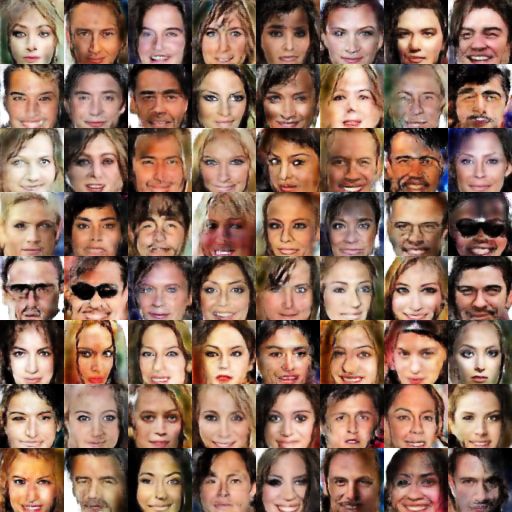
1. Introduction

   Generative models have been an active but challenging research field in tra-
ditional machine learning because of the intractability of many probabilistic
computations arising in approximating maximum likelihood estimation (MLE).
To avoid these computations, Generative Adversarial Network (GAN) [1] greatly
improves the quality of generated images by implicitly modeling the target dis-
tribution via neural networks instead of approximation of intractable likelihood
functions in capturing data distribution. To better utilize the information about
data structure in labeled data, Conditional GAN (CGAN) [2] feeds real labels
along with images and generate more realistic images. Unfortunately, CGAN
and subsequent extensions [3, 4, 5, 6, 7] suffer from a challenge that they require
large amounts of labeled data which is expensive or even impossible to acquire
in practice.
   To decrease the dependence of GANs on labeled data, it would be nicer to
find a substitution to replace the role of real labels. It is well known that
representation learning enables machine learning models to get more infor-
mation about data structure and class distribution. A commonly and widely
used method in representation learning is to employ K-Means. Recent works
[8, 9, 10, 11] have improved clustering results through jointly training K-Means
and deep neural networks. By fusing K-Means with the powerful nonlinear
expressiveness of neural networks, they get “K-Means-friendly” [9] representa-
tions, i.e., features that are more representative for clustering tasks. But most
of these neural networks are realized by a pre-trained auto-encoder on large-
scale datasets like ImageNet, which means they still utilize prior knowledge
(real-label) supervision.
   Inspired by the success of jointly training of neural networks and K-Means
on clustering tasks, Variational deep embedding (VaDE) [12] and Joint Gen-
erative MomentMatching Network (JGMMN) [13] instead combine generative
models with clustering methods and achieve competitive results not only on
clustering, but also on generating tasks. More specifically, VaDE proposes con-

                                        2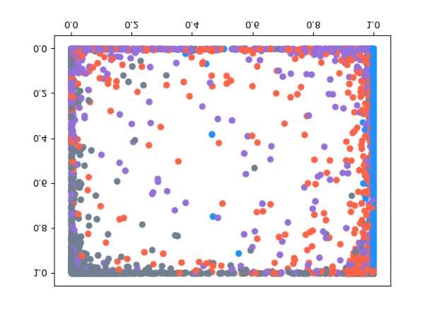
tinuous clustering objectives for Variational Autoencoder (VAE) [14] and JG-
MMN augments original loss functions of Generative Moment Matching Net-
works (GMMN) [15] with regularization terms to constrain latent variables. On
the other hand, authors of [16] perform K-Means on features of the top layer of
discriminators in GAN and Info-GAN [17] respectively and show that features
of Info-GAN are obviously more “K-Means-friendly” than regular GAN. This
implies that constrains on the latent space of GANs induce more representative
features. Furthermore, extensions of GANs [18, 19] give state-of-the-art results
on clustering by fusing GANs with clustering methods. Although these works
have achieved exciting results on clustering results by combining advantages of
GANs and clustering method, utilizing clustering methods to improve the qual-
ity of generating images of GANs also deserves more attentions. This brings the
main motivation of our work: Can we re-design the framework of GANs
in an un-conditional manner and utilize the capability of K-Means on
representation learning to replace the role of real labels?
   In order to make use of clustering labels of K-Means to direct the gener-
ating process as real labels in GANs, we consider operating K-Means on the
top layer of the discriminator. But the main difficulty is how to deal with the
un-differentiable objective of K-Means using Stochastic Gradient Decent (SGD)
[20]. Deep Embedded Clustering (DEC) [8] straightforwardly separates the
optimization into updating centers and network parameters successively. An-
other CNN-based method [21] also adopts this technique and further proposes
a feature drift compensation scheme to mitigate the drift error caused differ-
ent optimization direction of K-Means and regular loss functions. Then Deep
Clustering Network (DCN) [9] introduces a defined “pretext” objective, a math-
ematical combination of reconstruction loss and K-Means clustering objective,
and optimize K-means with back-propagation. Quite recently, Deep K-Means
[22] proposes a continuous reparametrization of the objective of K-Means clus-
tering to optimize it with SGD.
   Motivated by these works, we propose an un-conditional generative adver-
sarial model, named K-Means-GAN (KM-GAN), which embeds the idea of up-

                                       3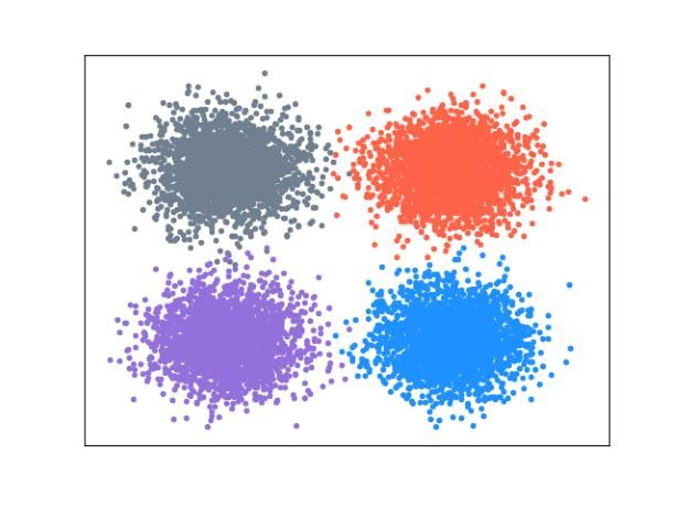
dating centroids of K-means into the framework of GANs. As the illustration
of the framework of our model in Fig. 1, it conducts the discriminator as a non-
linear feature extractor and utilizes K-Means clustering algorithm for getting
more representative features. Further, we employ obtained results of K-Means
instead of one-hot real labels to direct the generator in the generating process.
Then we propose objectives containing clustering labels from the perspective of
deep metric learning (DML) to let the optimization direction of K-Means agree
with the generating process. The specific optimization process includes three
terms to alternately optimize, of which the “center-loss” term tries to pull the
corresponding centers of real and generated images closer. Furthermore, the
objective of the discriminator is to minimize the distance between real samples
and their corresponding centers and maximize the distance between fake sam-
ples and their corresponding real centers. Meanwhile, the loss function of the
generator, which is interpreted as an adversarial term, attempts to approximate
the target distribution by decreasing the distance between generated samples
and their corresponding real centers.

                                                                          The First Forward to Get Clustering Label
                       ···
                              ···
                 ···

                                        ···

     Noise          Generator(MLP/CNN)
                                                                              ···
                                                         ···
                                                                    ···
                                              ···

                                              Feature Extractor(Discriminator MLP/CNN)         Feature           Clustering(K-Means)
                                                                                  Clustering Label

                                                                         The Second Forward to Get the Loss
                       Input Pictures                                                                                 Loss Function

Figure 1: The framework of KM-GAN. Notice that the first forward pass is to get the clustering
labels. In the second forward pass, the clustering labels and data are feeded to back-propagate
the obtained loss functions.

    Contribution To the best of our knowledge, our work is the first to at-
tempt to combine training unsupervised K-Means algorithm with GAN model

                                                     4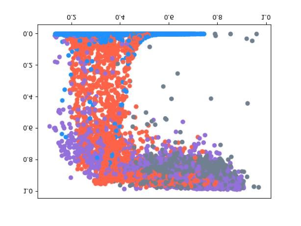
simultaneously through SGD for generating tasks. Our main contributions are
summarized as follows:

   • We propose an un-conditional implementation of GANs, called K-Means-
     GAN (KM-GAN), and equip it with new objective functions from the
     perspective of DML.

   • We incorporate GANs with the idea of traditional K-Means and utilize
     obtained labels, replacing the role of real labels, to direct the generating
     process and get more representative features.

   • We empirically show that KM-GAN is capable to generate diverse samples
     and the quality of generated images on several real datasets is competitive
     to that of conditional GANs.

2. Background

   In this section, we introduce notations and briefly review preliminary knowl-
edge, including the framework of GANs and K-Means. The notations provided
in this section will also be used in subsequent sections.

2.1. Notations

   Throughout the paper, we use b for the batch size, D for the discriminator,
G for the generator and k for the pre-defined number of classes.

2.2. Framework of GANs

   GAN [1] consists of two components: a discriminator D and a generator
G which are both realized by the neural networks. The main idea is actually
an adversarial training procedure between them. Throughout the adversarial
training, the generator G maps samples from a prior noise distribution, such
as gaussian distribution, to the data space while the discriminator D estimates
the probability that its inputs coming from real data distribution rather than
generated distribution.

                                        5
More specifically, given a noise distribution Pz and training samples x ∼ Px ,
the adversarial training contains two steps. Firstly, the generator maps noises z
from Pz to G(z) and update parameters of the discriminator while fix parameters
of the generator by optimizing the objective of D as follows:

                min Ex∼px [log D(x)] + Ez∼pz [log(1 − D(G(z)))].               (1)
                 D

   Then fix parameters of D and update parameters of G to approximate target
distribution by optimizing the loss function of G as follows:

                          max Ez∼pz [log(1 − D(G(z)))].                        (2)
                           G

   In order to generate more realistic images, CGANs [2] implements GANs
with one-hot real labels, which provides supplementary information of class dis-
tribution for generating process. This method qualitatively and quantitatively
improve the performance in generating tasks. Recent works [23, 24] then extend
VAE and GMMN based on this technique for more realistic images. Further-
more, Deep Convolutional GAN (DCGAN) [4] designs a stable architecture
utilizing convolutional neural networks and raises several tricks to stabilize the
adversarial training process. On the other hand, lots of works [5, 3, 25, 26, 27]
propose objectives for GANs to improve stability and image quality.

2.3. K-Means
   K-Means [28] is a traditional clustering method used to group a set of given
data points {xi }i=1,2,...,N ∈ Rm into k clusters, where k is a pre-defined number.
After randomly choosing k points of data samples as initialized center, the main
algorithm is composed of two steps. The first is to assign clustering labels to
each point according to the Euclidean distance between the point and current
the k centers. Then update new centers as the weighted average of points in
each class. The algorithm stops until each center do no change. Formally, the
cost function is as follows:
                                      N
                                      X
                          min               kxi − Msi k22
                     M∈Rm∗k ,si ∈Rk
                                      i=1                                      (3)
                                                     T
                               s.t.   sij ∈ {0, 1}, 1 si = 1, ∀i, j,

                                             6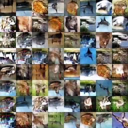
where si is the one-hot clustering label of data point xi , sij denotes the jth
element of vector si and M is a matrix, whose k columns correspond to the k
centers.
   As we can see from this formula, the performance of K-Means depends on
both features and initialized centers. So K-Means++ [29] is proposed to initial-
ize centers with a better procedure. Extensions [21, 22, 16] adopt the procedure
and achieve surprising results. Then to deal with large-scale datasets and online
scenarios, Minibatch K-Means [30] proposes to use a batch of samples to update
centers in each iteration.

3. Proposed Method

   As mentioned before, we consider re-designing the framework of GANs and
utilize results of K-means to replace the role of one-hot real labels in a un-
conditional manner. So we treat the discriminator as a feature extractor instead
of a classifier and operate K-Means on extracted features to produce clustering
labels which are viewed as substitution of real labels. With the obtained features
and labels, we propose our objectives from the perspective of DML to carry out
adversarial learning. More importantly, we come up with a “center-loss” term
to connect the optimization of adversarial learning and centers updating in K-
Means. In the following subsections, we first introduce proposed objectives and
optimization procedure in regular K-Means-GAN (KM-GAN). Then generalize
it with regularization terms in order to deal with more general datasets.

3.1. Regular KM-GAN

   We first introduce the “center-loss” term since it fills the gap between two
different optimization procedures of adversarial learning and K-Means, which is
important for the whole algorithm to work effectively. The term is interpreted
as a role to decrease the distance between corresponding centers of real and

                                        7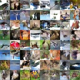
generated images. Formally, the formula is as follows:
                     k       Pjcm                  k       Pjcbm
                    X   cm + j=1    D(xnj,cm ) X       cm + j=1
                                                       b         D(G(znj,bcm ))
min     Lcenter = k                            −                                k1
D,G
                    m=1
                               1 + jcm            m=1
                                                             1 + jbcm

s.t.    Lcenter ≥ dround ,
                                                                               (4)

where k is the pre-defined number of classes, cm (b
                                                  cm ) is the m-th center of
features of real data (generated data) updated after last iteration, jcm (jbcm ) is
the number of features belonging to the center cm (b
                                                   cm ), nj,cm (nj,bcm ) denotes
the position of corresponding feature of real data (generated data) that is in
class m according to results of K-Means in the first forward pass and dround
is a hyperparameter needed to tune according to different datasets to avoid
degeneration.
   Indeed, Lcenter calculates the difference of second order statistical magni-
tude, i.e., the average of k centers, between features of real and generated im-
ages. The intension is to keep centers of synthesized data not far away from
that of real data and accelerate distribution approximation. The exploration of
minimizing statistical magnitudes is motivated by improvements of recent works
[31, 5, 15] on classification and generation tasks. Especially, GMMN success-
fully approximates data distribution through minimizing all orders of statistics,
which is realized by the Gaussian kernel. So we intuitively utilize the second or-
der statistics and reuse the results of K-Means to propose the continuous term.
Experiments further show that KM-GAN fails to generate meaningful images
even on MNIST without “center-loss” term.
   Although the “center-loss” term is proposed to approximate the target dis-
tribution, we still need objective functions for the discriminator and the gener-
ator to finish the regular adversarial training. Firstly, we define the objective
function of discriminator as follows:

                min   LD = kD(x) − Creal k2 − kD(G(z)) − Cgen k2 ,             (5)
                D

where Creal (Cgen ), computed based on real centers, consists of b center pieces
for the pre-defined batch size b. Each of these center pieces is the centroid of

                                        8
the real class that the feature piece in the corresponding position of this batch
belongs to. It’s natural to see that LD penalizes the distance between each
class of real data and their corresponding k centers. The interpretation is to
minimize intra-class distance of each class in the feature space of real data from
the viewpoint of DML. On the contrary, LD maximizes the distance between
generated data and centers of their corresponding real classes to discriminate
the counterfeit from real data.
   On the other hand, the corresponding objective function of the generator is
defined as follows:

                        min   LG = kD(G(z)) − Cgen k2 .                       (6)
                         G

   Obviously, the effect of the objective is to compete with the discriminator
to approximate the target distribution. When decreasing the distance between
synthesized data and centers of their corresponding k real classes, the features
of generated images are distributed around each real center like features of real
data. Then with the impact of “center-loss” to pull centers of real and fake data
close, fake data distribution would approximate target distribution finally. The
term also plays a role as an adversarial term in the framework of KM-GAN.

3.2. Three-Step Alternating Optimization

   Optimizing network parameters of GANs and updating centers step by step
is straightforward as in DEC [8]. But the different directions of these two steps
make the optimization more difficult. To deal with this issue, we utilize “center-
loss” term to bridge the gap. Especially, the “center-loss” term reuses results
of K-Means and obtained features from the discriminator, which builds a con-
nection between these two steps. In the specific optimization, we first solve the
subproblem of adversarial learning, i.e., updating parameters of the discrimi-
nator and generator, respectively. Then inspired by alternating optimization
in [9], we utilize “center-loss” to re-update parameters of D and G via SGD.
With current parameters, we obtain centers in feature space at last by Equa-
tion 3. The concretely three-step alternating optimization procedure is shown

                                        9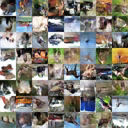
Algorithm 1 Training algorithm for regular KM-GAN
Input: Real images X, noise distributionPZ , pre-defined number of classes k,
  number of iterations T , batch size b and hyper-parameters of Adam α, β1 , β2
Output: Generated samples G(z)
  Initialize parameters of D and G networks
  Initialize k real centers of mapped features D(X) by K-Means++
  for t = 1 : T do
    Sample a batch {xi }bi=1 from real data X
    Sample a batch {zi }bi=1 from noise distribution PZ
    Obtain features {D(xi )}bi=1 and {D(G(zi ))}bi=1
    Obtain clustering labels according to Euclidean distance with current k
    centers
    gradθd = Oθd LD
    θd =Adam(gradθd , θd , α, β1 , β2 )
    gradθg = Oθg LG

    θg =Adam(gradθg , θg , α, β1 , β2 )
    gradθd ,θg = Oθd ,θg Lcenter
    θd , θg =Adam(gradθd ,θg , θd , θg , α, β1 , β2 )

    Update centers via K-Means objective in Equation 3
  end for

                                             10
in Algorithm 1.
In the described algorithm, we conduct K-Means++ technique to better
initialize centers of features. In addition, since the optimization of network
parameters employs Adam [20] and depends on the pre-defined batch size, it’s
natural to come up with Minibatch K-Means. With this procedure, the “center-
loss” further plays a role to mitigate the error caused different optimization
direction of K-Means and regular loss functions in each iteration of a whole
epoch similar to [21].
3.3. Generalized KM-GAN
Although common used datasets have obvious criterions to cluster, such as
MNIST [32] and CIFAR-10 [33]. However, there exist datasets that do not have
these obvious criterions. For example, CelebA [34] and LFW [35] contains too
many personalities and images for each personality are not enough for generation
tasks. It’s even hard to find a suitable number for the pre-defined k. In this
case, operating K-Means to cluster features is too difficult. To handle with
such problem, we generalize regular KM-GAN with two regularization terms.
They act as constraints [5] on the whole class of real and fake images. Before
explaining the constraints, we define two necessary terms Lintra and Linter used
to generalize KM-GAN as follows:
X X
Lintra = kD(xi ) − D(xj )k1 + kD(G(zi )) − D(G(zj ))k1 ,
xi ,xj ∈Bd G(zi ),G(zj )∈Bg
X
Linter = kD(xi ) − D(G(zj )))k1 ,
xi ∈Bd ,G(zj )∈Bg
b
where Bd and Bg denote the corresponding batch of real samples {xi }i=1 and
b
generated samples {G(zi )}i=1 , respectively.
Then the objective functions of the discriminator and the generator become:
LD = min kD(X) − Creal k2 − kD(G(z)) − Cgen k2 + λ ∗ (Lintra − Linter ),
θD
(7)
LG = min kD(G(z)) − Cgen k2 + λ ∗ Linter .
θG
11In the case described above, the objective functions of regular KM-GAN
are not effective enough since they are dependent on k. However these two
terms, one decreases intra-class distances of the whole real and fake data in
feature space while the other minimizes inter-class distance to approximate data
distribution, help to approximate the data distribution as a whole class. With
above regularization terms, experimental results also show that the final centers
reduce to the same one whatever the pre-defined k is (such as k = 10 or k =
20), which coincides with the goal of these regularization terms. This implies
that KM-GAN could adapt to more general scenarios with them. We use the
hyperparameter λ in experiments to balance the regular loss functions and these
two regularization terms.
4. Experiments
In this section, we first conduct experiments on a synthetic dataset to show
the capability of the discriminator of KM-GAN to represent features. Then
we qualitatively and quantitatively show that KM-GAN is able to generate
realistic and diverse images on real-world datasets including MNIST, Fashion-
10, CIFAR-10 and CelebA. Details about these datasets are shown in Table ??.
Note that the hyperparameter λ is set to 0 in experiments except CelebA, where
it is set to 5.
Dataset Numbers of Images Feature Dimensions Classes
Synthesis 10,000 100 4
MNIST 70,000 28×28 10
Fashion-10 70,000 28×28 10
CIFAR-10 70,000 32×32×3 10
CelebA 202,599 64×64×3 No
Table 1: Details of synthetic data and real-world datasets.
12(a) Real data (b) Epoch 0 (c) Epoch 50 (d) Epoch 150 (e) Epoch 200
Figure 2: Subfigure (a) is the visualization of intrinsic 2-dimension structure of synthetic data.
Subfigures (b)-(e) are visualization of features on the top layer of corresponding discrimina-
tors of DCGAN and KM-GAN in the training process on synthetic dataset. The four kinds
of colored points represent different categories. Obviously, the features of KM-GAN could
separate most of them while that of DCGAN is ineffective.
4.1. KM-GAN on Synthetic Data
As we can see from loss functions of KM-GAN, features of the discriminator
play an important role not only on the objective function of the discriminator
itself, but also on that of the generator. To demonstrate that features of KM-
GAN are really representative, we compare with that of DCGAN which shows its
capability to do representation learning by conducting classification experiments
using its trained discriminator. The obtained features of KM-GAN and DCGAN
on a synthetic dataset in the training process are shown in Fig. 2.
The synthetic dataset consists of 10, 000 points that belong to R100 and has
“K-Means-friendly” [9] structure in a two-dimensional domain which we could
not observe. In fact, we first choose four two-dimensional gaussian distributions
with different means and covariance matrices as in Fig. 2a. Then sample 2, 500
points from each distribution and map them into R100 through a mapping func-
tion M, which is realized by a non-linear neural network showed in Table 4.1. In
this experiment, we set dround as 0, and the network structures of DCGAN[1]
and KM-GAN are the same and both shown in Table 4.1. The visualization
of the features learned in the training process by discriminators of these two
models are showed in Fig. 2. Compared with features of DCGAN, those of
13our proposed KM-GAN are obviously more representative to show the intrinsic
structure although they are both capable to generate high-quality images on
real-world datasets.
Mapping function M Generator Discriminator
n n n
Input {hi }i=1 ∈ R2 Input {zi }i=1 ∈ R100 Input {xi }i=1 ∈ R100
FC 10 Sigmoid FC 10 ReLU BN FC 100 ReLU BN
FC 100 Sigmoid FC 50 ReLU BN FC 50 ReLU BN
n 100
{xi }i=1 ∈R FC 100 ReLU BN FC 10 ReLU BN
n
{G(zi )}i=1 ∈ R100 FC 2 Sigmoid
n
{D(xi ), D(G(zi ))}i=1 ∈ R2
Table 2: Architectures of M, generator and discriminator.
4.2. KM-GAN on MNIST
MNIST [32] dataset has 70, 000 gray images of handwritten digits of size
28 × 28. We first conduct experiments to compare KM-GAN with its reduced
version which operates K-Means in pixel space as introduced in Algorithm 2.
Then we improve KM-GAN with weight-clipping which stabilizes the training
process. The network structures of KM-GAN for training MNIST are the same
as that of DCGAN and hyperparameter dround is set as 10, 000.
4.2.1. Feature Space vs. Original Space
To demonstrate the effect of carrying out K-Means in feature space rather
than pixel space, we compare KM-GAN with reduced KM-GAN, in which we
operate K-Means in pixel space and cluster original data. Indeed, computations
in K-Means appear to increase quickly as the dimensionality of data increases
when experimenting with reduced KM-GAN. However, the capability of dimen-
sionality reduction of KM-GAN avoids such computational difficulties. In the
following, we further qualitatively show the advantage of operating K-Means on
latent space as exhibited images in Fig. 3.
From images in Fig. 3b and Fig. 3c, it is obvious that the quality of
generated digits is significantly better when clustering is operated in the feature
14Algorithm 2 Training algorithm for reduced KM-GAN
Input: Real Images X, noise distributionPZ , pre-defined number of classes k,
number of iterations T , batch size b and hyper-parameters of Adam α, β1 , β2
Output: Generated samples G(z)
Initialize k real centers C
e of data X by K-Means++
Initialize parameters of D and G networks
for t = 1 : T do
Sample a batch {xi }bi=1 from real data X
Sample a batch {zi }bi=1 from noise distribution PZ
Obtain features {D(xi )}bi=1 and {D(G(zi ))}bi=1
Obtain clustering labels according to Euclidean distance with current k
centers
e center = kD(C
L ereal ) − D(C
egen )k1
gradθd ,θg = Oθd ,θg L
e center
θd , θg =Adam(gradθd ,θg , θd , θg , α, β1 , β2 )
e D = kD(x) − D(C
L ereal )k2
gradθd = Oθd L
eD
θd =Adam(gradθd , θd , α, β1 , β2 )
e G = kD(G(z)) − D(C
L egen )k2
gradθg = Oθg L
eG
θg =Adam(gradθg , θg , α, β1 , β2 )
Update centers in original pixel space via K-Means objective in Equation 3
end for
15(a) Real data (b) Reduced KM-GAN (c) KM-GAN
Figure 3: Comparison of generated samples of KM-GAN and reduced version of KM-GAN on
MNIST dataset.
space. Regular KM-GAN successfully generates realistic handwritten digits not
only in different classes and angles while reduced KM-GAN even suffers mode
collapse, i.e., most of generated images are similar or identical.
4.2.2. Improvement on KM-GAN
Although KM-GAN is proven to be capable to generate realistic and diverse
images, it still fails to generate images sometimes. So we utilize a common
technique called weight clipping to constrain parameters of the discriminator
(feature extractor). Specifically, we clamp the weights of D to a fixed box
so that it could only output values in a certain range. The technique further
guarantees the property that points close in pixel space are not far away from
each other after mapped into feature space.
As synthesized images shown in Fig. 4a and Fig. 4b, the performance of KM-
GAN without weight clipping is already competitive with DCGAN on MNIST
dataset. This demonstrates that the utilization of clustering labels successfully
replaces the role of real labels to direct generating process and encourages us
to pay more attention to un-conditional generative models. What’s more, to
stabilize the three-step alternating optimization process, we equip KM-GAN
with weight clipping and the clipping threshold is set to [−1, 1]. The synthesized
images shown in Fig. 4c are competitive or even better than KM-GAN without
16(a) DCGAN (b) KM-GAN (c) KM-GAN with weight
clipping
Figure 4: Subfigures (a) and (b) compare generated images of DCGAN and KM-GAN on
MNIST dataset, and subfigure (c) shows generated images of KM-GAN improved with weight
clipping.
weight clipping.
4.3. KM-GAN on Fashion-10
Fashion-10 dataset, consisting of various types of more complicated fashion
products rather than handwritten digits, has the same number of images as
MNIST and the size of each image is also 28×28. So we use the same architecture
as used on MNIST to examine KM-GAN on Fashion-10. The hyperparameter
dround is also the same as on MNIST. From the experimental results shown
in Fig. 5a and Fig. 5b, the quality of synthesized images of KM-GAN is
comparable to that of DCGAN.
To further quantitatively show that our proposed method is also capable to
generate diverse images without the help of one-hot real labels, we train a three-
layer convolutional classifier on Fashion-10 separately (97% accuracy on training
set and 91% on test set) and use the classifier to classify 5, 000 synthesized
images of KM-GAN and DCGAN. The result of the frequency of each class is
shown in Fig. 5c. Indeed, since Fashion-10 equally contains images of each
class, conditional models easily generate images equally for each class with the
help of real labels. So we compare with results of DCGAN to further show that
KM-GAN is also capable achieve this. Specifically, in the frequency chart of
17(a) DCGAN (b) KM-GAN (c) Frequency chart
Figure 5: Evaluation of synthesized images of KM-GAN on Fashion-10 dataset. Subfigures (a)
and (b) exhibit a random batch of generated images of DCGAN and KM-GAN, and subfigure
(c) shows the distributions of generated images of DCGAN and KM-GAN, respectively.
generated images, numbers 0 ∼ 9 denote 10 classes of the dataset and two colors,
“blue” and “gray”, represent results of KM-GAN and DCGAN, respectively.
From the class distributions, most classes are generated with probability close
to 10% by KM-GAN except the class “shirts”, which is under-represented with
7.0%. We infer this is because that “shirts” are very similar to “T-shirts” and
“pullovers”.
4.4. KM-GAN on CIFAR-10
CIFAR-10 [33] is a dataset with 60, 000 RGB images of size 32 × 32 in 10
classes. There are 6, 000 images in each class with 5, 000 for training and 1, 000
for testing. All these images are used here to train KM-GAN. The network struc-
tures are shown in Table 3 and we set dround to 20, 000 and clipping threshold
to [−0.01, 0.01].
We first evaluate the generated images of KM-GAN on CIFAR-10 dataset
and show the experimental results in Fig. 6. To demonstrate the capability of
our proposed objective functions, we compare with MBGAN which also proposes
different objective functions from the perspective of DML. Results shows that
synthesized images of KM-GAN are obviously more realistic and meaningful.
We further compare with DCGAN and there is no visual difference between the
quality of synthesized images of these two models, which again demonstrates
18the effectiveness of KM-GAN.
Table 3: Architectures of generator and discriminator on CIFAR-10.
Generator Discriminator
n n
Input {zi }i=1 ∈ R100 Input {xi }i=1 ∈ R64×64×3
FC 4 × 4 × 512 BN ReLU 5 × 5 Conv
64 stride 2 ReLU
5 × 5 Upconv 5 × 5 Conv
256 stride 2 BN ReLU 128 stride 2 BN ReLU
5 × 5 Upconv 5 × 5 Conv
128 stride 2 BN ReLU 256 stride 2 BN ReLU
5 × 5 Upconv 5 × 5 Conv
64 stride 2 BN ReLU 512 stride 2 BN ReLU
5 × 5 Upconv FC 4096 BN ReLU
3 Stride 2 Sigmoid
FC 100 BN ReLU
Since we use clustering labels of K-Means to replace one-hot real labels in
KM-GAN, i.e., a purely un-supervised training, we quantitatively evaluate the
diversity of images synthesized by our model with another index called inception
score [36] on CIFAR-10 dataset. The index applies Inception model [37] to every
generated image and computes the following metric:
IS(G(z)) = exp(Ez KL(p(y|G(z))kp(y))). (8)
Indeed, the main idea of Equation 8 is that diverse generated images which
contain meaningful objects are supposed to have a conditional label distribution
R
p(y|G(z)) with low entropy and a marginal distribution p(y|G(z))dz with high
entropy. As in Table 4, we report inception scores of both conditional and un-
conditional models to characterize the performance of KM-GAN. Specifically,
WGAN, Improved GANs, and MIX+WGAN are trained without feeding real
labels, while ALI is itself an un-conditional model utilizing an auto-encoder to
assist the generator to approximate target distribution. Obviously, KM-GAN
19performs much better than these models which demonstrates the effectiveness
of KM-GAN. We then compare with two conditional methods based on DML,
MLGAN and MBGAN. KM-GAN also works better than than them. Further-
more, we compare with DCGAN, a very stable and common used conditional
method in the research field of GANs. Results show that KM-GAN are compa-
rable to DCGAN just like from above synthesized images. We infer that this is
because synthesized images of KM-GAN shown in Fig. 6c are more meaningful
while the backgrounds of generated images of DCGAN shown in Fig. 6b are
more clear.
Table 4: Inception Score on CIFAR-10 Dataset.
Model Inception Score
MBGAN 4.27 ± 0.07
Conditional MLGAN-clipping [5] 5.23 ± 0.29
Models DCGAN 5.37 ± 0.06
MIX + WGAN [38] 4.04 ± 0.07
Un-conditional Improved GANs [36] 4.36 ± 0.04
Models ALI [39] (from [40]) 4.79
Wasserstein GANs [25] (from [38]) 3.82 ± 0.06
KM − GAN 5.39 ± 0.05
(a) MBGAN (b) DCGAN (c) KM-GAN
Figure 6: Comparison of generated samples of MBGAN, DCGAN and KM-GAN on CIFAR-
10.
204.5. KM-GAN on CelebA
CelebA [34], as a large-scale face dataset, contains more than 200, 000 RGB
face images from 10, 177 celebrity identities, and there are 40 binary attributes
and 5 landmarks for each image. In this experiment, we crop images into 64×64,
and the network structures are shown in Table 5. The hyperparameters dround
and clipping threshold are set the same as in CIFAR-10 dataset. Besides, we
set λ set as 5 since we could not find an appropriate k for this CelebA while
other datasets have determinate categories. Following are samples generated by
DCGAN and KM-GAN, respectively.
Table 5: Architectures of generator and discriminator on CelebA.
Generator Discriminator
n n
Input {zi }i=1 ∈ R100 Input {xi }i=1 ∈ R64×64×3
FC 4 × 4 × 512 BN ReLU 5 × 5 Conv
64 stride 2 BN ReLU
5 × 5 Upconv 5 × 5 Conv
256 stride 2 BN ReLU 128 stride 2 BN ReLU
5 × 5 Upconv 5 × 5 Conv
128 stride 2 BN ReLU 256 stride 2 BN ReLU
5 × 5 Upconv 5 × 5 Conv
128 stride 2 BN ReLU 512 stride 2 BN ReLU
5 × 5 Upconv FC 100 Sigmoid
3 Stride 2 Tanh
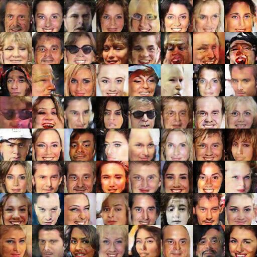
From results in Fig. 7, we see that KM-GAN also works well on CelebA.
Then we interpolate synthesized images to demonstrate the generalization ca-
pability of KM-GAN rather than only generating the training face images. We
first interpolate z ∈ R100 and then map interpolated z with the generator.
The results are as shown in Fig. 8. The leftmost and rightmost images are
mapped from z0 and z1 , respectively. The other images are generated from
zβ = βz0 + (1 − β)z1 (β ∈ [0, 1]), i.e., interpolations of corresponding noise vec-
tors. As examples in Fig. 8, generated images change smoothly from leftmost
21(a) DCGAN (b) KM-GAN
Figure 7: Comparison of generated samples of DCGAN and KM-GAN on CelebA.
to rightmost. Indeed, we choose features of faces, including hair color, angles
of faces, with or without eyeglasses and some other special features, to exhibit
the continuous change clearly. Especially, on the first row, the face of a smiling
woman with golden hair transitions to the face of a seriously man with dark hair
slowly. In addition, on the second row, the face of a woman with dark hair and
close mouth changes to the face of a smiling woman with golden hair. These
interpolations indicate that our proposed KM-GAN is able to generate images
continuously instead of only memorizing training data.
22Figure 8: Interpolations of generated images on CelebA dataset.
5. Conclusion
In this paper, we propose an un-conditional extension of GANs, called KM-
GAN, by fusing with the idea of K-Means and utilizing the clustering results
to propose objective functions that direct the generating process. The purpose
is to replace the role of one-hot real labels with the clustering results, which
generalizes GANs to applications where real labels are expensive or impossible
to obtain. In addition, we conduct experiments on several real-world datasets
to demonstrate that KM-GAN is really capable to generate realistic and diverse
images without mode collapse. In the future, we would further pay attention
to proving the positive correlation between high-quality synthesized images and
high clustering accuracy and utilize the relationship to improve performance of
both tasks.
Acknowledgments
The authors would like to thank Jiaxiang Guo, Tianli Liao, Yifang Xu,
Bowen Wu, Mengya Zhang, Chengdong Zhao and Dong Wang for their helpful
advices.
References
References
[1] I. Goodfellow, J. Pouget-Abadie, M. Mirza, B. Xu, D. Warde-Farley,
S. Ozair, A. Courville, Y. Bengio, Generative adversarial nets, in: Ad-
vances in neural information processing systems, 2014, pp. 2672–2680.
[2] M. Mirza, S. Osindero, Conditional generative adversarial nets, arXiv
preprint arXiv:1411.1784.
23[3] G. Dai, J. Xie, Y. Fang, Metric-based generative adversarial network, in:
Proceedings of the 2017 ACM on Multimedia Conference, ACM, 2017, pp.
672–680.
[4] A. Radford, L. Metz, S. Chintala, Unsupervised representation learning
with deep convolutional generative adversarial networks, arXiv preprint
arXiv:1511.06434.
[5] Z.-Y. Dou, Metric learning-based generative adversarial network, arXiv
preprint arXiv:1711.02792.
[6] X. Mao, Q. Li, H. Xie, R. Y. Lau, Z. Wang, S. P. Smolley, Least squares
generative adversarial networks, in: Computer Vision (ICCV), 2017 IEEE
International Conference on, IEEE, 2017, pp. 2813–2821.
[7] X. Huang, Y. Li, O. Poursaeed, J. Hopcroft, S. Belongie, Stacked genera-
tive adversarial networks, in: IEEE Conference on Computer Vision and
Pattern Recognition (CVPR), Vol. 2, 2017.
[8] J. Xie, R. Girshick, A. Farhadi, Unsupervised deep embedding for clustering
analysis, in: International conference on machine learning, 2016, pp. 478–
487.
[9] B. Yang, X. Fu, N. D. Sidiropoulos, M. Hong, Towards k-means-friendly
spaces: Simultaneous deep learning and clustering, in: International Con-
ference on Machine Learning, 2017, pp. 3861–3870.
[10] J. Yang, D. Parikh, D. Batra, Joint unsupervised learning of deep repre-
sentations and image clusters, in: Proceedings of the IEEE Conference on
Computer Vision and Pattern Recognition, 2016, pp. 5147–5156.
[11] E. Aljalbout, V. Golkov, Y. Siddiqui, D. Cremers, Clustering with deep
learning: Taxonomy and new methods, arXiv preprint arXiv:1801.07648.
[12] Z. Jiang, Y. Zheng, H. Tan, B. Tang, H. Zhou, Variational deep embedding:
an unsupervised and generative approach to clustering, in: Proceedings of
24the 26th International Joint Conference on Artificial Intelligence, AAAI
Press, 2017, pp. 1965–1972.
[13] H. Gao, H. Huang, Joint generative moment-matching network for learning
structural latent code., in: IJCAI, 2018, pp. 2121–2127.
[14] D. P. Kingma, M. Welling, Auto-encoding variational bayes, arXiv preprint
arXiv:1312.6114.
[15] Y. Li, K. Swersky, R. Zemel, Generative moment matching networks, in:
International Conference on Machine Learning, 2015, pp. 1718–1727.
[16] V. Premachandran, A. L. Yuille, Unsupervised learning using generative
adversarial training and clustering.
[17] X. Chen, Y. Duan, R. Houthooft, J. Schulman, I. Sutskever, P. Abbeel,
Infogan: Interpretable representation learning by information maximizing
generative adversarial nets, in: Advances in neural information processing
systems, 2016, pp. 2172–2180.
[18] M. Ben-Yosef, D. Weinshall, Gaussian mixture generative adversarial net-
works for diverse datasets, and the unsupervised clustering of images, arXiv
preprint arXiv:1808.10356.
[19] S. Mukherjee, H. Asnani, E. Lin, S. Kannan, Clustergan: Latent space clus-
tering in generative adversarial networks, arXiv preprint arXiv:1809.03627.
[20] D. P. Kingma, J. Ba, Adam: A method for stochastic optimization, arXiv
preprint arXiv:1412.6980.
[21] C.-C. Hsu, C.-W. Lin, Cnn-based joint clustering and representation learn-
ing with feature drift compensation for large-scale image data, IEEE Trans-
actions on Multimedia 20 (2) (2018) 421–429.
[22] M. M. Fard, T. Thonet, E. Gaussier, Deep k-means: Jointly clustering with
k-means and learning representations, arXiv preprint arXiv:1806.10069.
25[23] C. Doersch, Tutorial on variational autoencoders, arXiv preprint
arXiv:1606.05908.
[24] Y. Ren, J. Zhu, J. Li, Y. Luo, Conditional generative moment-matching
networks, in: Advances in Neural Information Processing Systems, 2016,
pp. 2928–2936.
[25] M. Arjovsky, S. Chintala, L. Bottou, Wasserstein generative adversarial
networks, in: International Conference on Machine Learning, 2017, pp.
214–223.
[26] S. Nowozin, B. Cseke, R. Tomioka, f-gan: Training generative neural sam-
plers using variational divergence minimization, in: Advances in Neural
Information Processing Systems, 2016, pp. 271–279.
[27] G.-J. Qi, Loss-sensitive generative adversarial networks on lipschitz densi-
ties, arXiv preprint arXiv:1701.06264.
[28] J. MacQueen, et al., Some methods for classification and analysis of mul-
tivariate observations, in: Proceedings of the fifth Berkeley symposium on
mathematical statistics and probability, Vol. 1, Oakland, CA, USA, 1967,
pp. 281–297.
[29] D. Arthur, S. Vassilvitskii, k-means++: The advantages of careful seed-
ing, in: Proceedings of the eighteenth annual ACM-SIAM symposium on
Discrete algorithms, Society for Industrial and Applied Mathematics, 2007,
pp. 1027–1035.
[30] D. Sculley, Web-scale k-means clustering, in: Proceedings of the 19th in-
ternational conference on World wide web, ACM, 2010, pp. 1177–1178.
[31] Y. Wen, K. Zhang, Z. Li, Y. Qiao, A discriminative feature learning ap-
proach for deep face recognition, in: European Conference on Computer
Vision, Springer, 2016, pp. 499–515.
26[32] Y. LeCun, L. Bottou, Y. Bengio, P. Haffner, Gradient-based learning ap-
plied to document recognition, Proceedings of the IEEE 86 (11) (1998)
2278–2324.
[33] Y. Netzer, T. Wang, A. Coates, A. Bissacco, B. Wu, A. Y. Ng, Reading
digits in natural images with unsupervised feature learning, in: NIPS work-
shop on deep learning and unsupervised feature learning, Vol. 2011, 2011,
p. 5.
[34] Z. Liu, P. Luo, X. Wang, X. Tang, Deep learning face attributes in the
wild, in: Proceedings of the IEEE International Conference on Computer
Vision, 2015, pp. 3730–3738.
[35] E. Learned-Miller, G. B. Huang, A. RoyChowdhury, H. Li, G. Hua, Labeled
faces in the wild: A survey, in: Advances in face detection and facial image
analysis, Springer, 2016, pp. 189–248.
[36] T. Salimans, I. Goodfellow, W. Zaremba, V. Cheung, A. Radford, X. Chen,
Improved techniques for training gans, in: Advances in Neural Information
Processing Systems, 2016, pp. 2234–2242.
[37] C. Szegedy, V. Vanhoucke, S. Ioffe, J. Shlens, Z. Wojna, Rethinking the
inception architecture for computer vision, in: Proceedings of the IEEE
conference on computer vision and pattern recognition, 2016, pp. 2818–
2826.
[38] S. Arora, R. Ge, Y. Liang, T. Ma, Y. Zhang, Generalization and equilibrium
in generative adversarial nets (gans), arXiv preprint arXiv:1703.00573.
[39] V. Dumoulin, I. Belghazi, B. Poole, O. Mastropietro, A. Lamb, M. Ar-
jovsky, A. Courville, Adversarially learned inference, arXiv preprint
arXiv:1606.00704.
[40] Y. Pu, W. Wang, R. Henao, L. Chen, Z. Gan, C. Li, L. Carin, Adversarial
symmetric variational autoencoder, in: Advances in Neural Information
Processing Systems, 2017, pp. 4330–4339.
27You can also read