Smooth Deep Image Generator from Noises - MIT alumni
←
→
Page content transcription
If your browser does not render page correctly, please read the page content below
Smooth Deep Image Generator from Noises
                       Tianyu Guo1,2,3 , Chang Xu2 , Boxin Shi4 , Chao Xu1,3 , Dacheng Tao2
                  1
                   Key Laboratory of Machine Perception (MOE), School of EECS, Peking University, China
              2
                UBTECH Sydney AI Centre, School of Computer Science, FEIT, University of Sydney, Australia
                             3
                               Cooperative Medianet Innovation Center, Peking University, China
             4
               National Engineering Laboratory for Video Technology, School of EECS, Peking University, China
                            tianyuguo@pku.edu.cn, c.xu@sydney.edu.au, shiboxin@pku.edu.cn,
                                    xuchao@cis.pku.edu.cn, dacheng.tao@sydney.edu.au

                            Abstract
  Generative Adversarial Networks (GANs) have demonstrated
  a strong ability to fit complex distributions since they were
  presented, especially in the field of generating natural images.
  Linear interpolation in the noise space produces a continu-
  ously changing in the image space, which is an impressive
  property of GANs. However, there is no special consideration
  on this property in the objective function of GANs or its de-           (a) Interpolation image shows blur and distorted images.
  rived models. This paper analyzes the perturbation on the in-
  put of the generator and its influence on the generated images.
  A smooth generator is then developed by investigating the
  tolerable input perturbation. We further integrate this smooth
  generator with a gradient penalized discriminator, and design
  smooth GAN that generates stable and high-quality images.
  Experiments on real-world image datasets demonstrate the
  necessity of studying smooth generator and the effectiveness
  of the proposed algorithm.                                           (b) Smooth interpolation shows clear and high-quality images.

                        Introduction                                 Figure 1: Interpolation images generated from WGAN-GP
                                                                     (Gulrajani et al. 2017) (a) and the proposed smooth GAN
Deep generative models have attracted increasing attention           (b).
from researchers, especially in the task of natural image
generation. Representative techniques include Variational
Auto-Encoder (VAE) (Kingma and Welling 2013), Pixel-                 and Bottou 2017; Gulrajani et al. 2017). Besides, a consider-
CNN (van den Oord et al. 2016), and Generative Adver-                able body of work has been conducted to arbitrarily manip-
sarial Networks (GANs) (Goodfellow et al. 2014). Genera-             ulate generated images according to different factors, e.g.,
tive Adversarial Networks (GANs) (Goodfellow et al. 2014)            the category, illumination, and style (Chen et al. 2016). Be-
translate Gaussian inputs into natural images by discover-           yond meaningless noise input in GANs, interpretable fea-
ing the equilibrium within a max-min game. The genera-               tures can be discovered by investigating label information
tor in vanilla GANs is to transform noisy vectors into im-           in conditional GANs (Mirza and Osindero 2014), exploring
ages, while the discriminator aims to distinguish the gener-         the mutual information between elements of input in info-
ated samples from real samples. Convincing images gener-             GAN (Chen et al. 2016) or leveraging the discriminator on
ated from noisy vectors through GANs could be employed to            latent space in AAE (Makhzani et al. 2015).
augment image datasets, which would alleviate the shortage
                                                                        Noise vector inputs for GANs can be taken as low-
of training data in some tasks. Moreover, image-to-image
                                                                     dimensional representations of images. As widely accepted
translation (Chen et al. 2018; 2019) based on GANs also
                                                                     in representation learning, the closeness of two data points
gets its popularity.
                                                                     is supposed to be preserved before and after transforma-
   However, vanilla GANs have flaws in its stability, and
                                                                     tion. Most of these improved GANs methods implicitly as-
we have seen many promising works to alleviate this prob-
                                                                     sume that the generator would translate linear interpolation
lem by modifying the network frameworks or proposing im-
                                                                     in the input noise space to semantic interpolation in the out-
proved loss functions (Radford, Metz, and Chintala 2015;
                                                                     put image space (Bojanowski et al. 2017). Although this
Nguyen et al. 2017; Karras et al. 2017; Mao et al. 2017;
                                                                     kind of experimental result showing interesting visual ef-
Berthelot, Schumm, and Metz 2017a; Arjovsky, Chintala,
                                                                     fects attracts readers’ attention, the quality of images gener-
Copyright c 2019, Association for the Advancement of Artificial      ated through interpolations could be very noisy and fragile,
Intelligence (www.aaai.org). All rights reserved.                    and some of these images would look obviously unnatural
or even meaningless, as demonstrated in Figure 1(a). Efforts     al. 2017a) introduced a classifier C to perform generation
are spent towards generating high-quality images or stabiliz-    tasks under semi-supervised conditions. DCGAN (Radford,
ing the training of GANs, and how to ensure the success of       Metz, and Chintala 2015) introduced interpolation in latent
semantic interpolation in GANs has rarely been investigated.     space generate the smooth transition in image space. How-
   In this paper, we propose a smooth deep image gener-          ever, there is no insurance for the sign of smooth transition
ator that can suppress the influence of input perturbations      in the adversarial Loss. As a result, this paper analyzes the
on generated images. By investigating the connections be-        constraint required by the smooth transition in image space
tween input noises and generated images, we theoretically        and introduces a method to enhance this sign of GANs.
present the most serious input perturbation that can be tol-
erated for an output image of desired precision. A gradient-                         Proposed Method
based loss function is then introduced to reduce the variation   In this section, we analyze the conditions required by the
of generated images caused by perturbations on input noises,     smooth transition in image space and develop a smooth gen-
which encourages a smooth interpolation of images. Com-          erator within GANs.
bining a discriminator with gradient penalty, we show the
smooth generator will be beneficial for improving the qual-      Generative Adversarial Nets
ity of interpolation samples, as demonstrated in Figure 1(b).
Experimental results on real-world datasets MNIST (LeCun         A discriminator D and a generator G play a max-min game
et al. 1998), CIFAR-10 (Krizhevsky and Hinton 2009), and         in GANs, in which the discriminator D is responsible for
CelebA (Liu et al. 2015) demonstrate the generator pro-          distinguishing real samples from generated samples, while
duced by the proposed method is essential for the success        the generator G is to deceive the discriminator D. When the
of smooth and high-quality interpolation of images.              game achieves equilibrium, the generator G would be able
                                                                 to fit complicated distribution of real samples.
                     Related Work                                   Formally given the sample x from the real distribution
                                                                 Pd and the noise z drawn from noise distribution Pz (e.g.,
In this section, we briefly introduce related works on gener-    Gaussian or uniform distribution), the optimal generator G
ative adversarial networks (GANs).                               transforming the noise distribution to the real data distribu-
   Although the GANs model has powerful image genera-            tion can be solved from the following min-max optimization
tion capabilities, the model was often trapped in the prob-      problem:
lem of unstable training and difficulty in convergence. Some
methods have been proposed to solve this problem. DC-
GAN (Radford, Metz, and Chintala 2015) introduced a net-           min max E [log(D(x))] + E [log(D(G(z)))].               (1)
                                                                     G    D   x∼Pd                z∼Pz
work structure that works well and is stable. WGAN (Ar-
jovsky, Chintala, and Bottou 2017) proved the defect of          We denote the distribution of generated sample G(z) as PG .
vanilla adversarial loss and proposed Wasserstein distance       By alternately optimizing the generator G and the discrim-
to measure the distance between the generated data distri-       inator D in the min-max problem, we expect that the dif-
bution and the real data distribution. However, the weight       ference between the generated distribution PG and the real
clip used in WGAN to ensure the Lipschitz continuous of          data distribution Pd would be gradually consistent with each
D leads to the loss of the capacity of neural networks. To       other.
solve this problem, WGAN-GP (Gulrajani et al. 2017) pro-
posed gradient penalty instead of weight clip operation to       Smooth Generator
satisfy Lipschitz continuous condition. BEGAN (Berthelot,
Schumm, and Metz 2017a) proposed a novel concept of              In the noise-to-image generation task, it is difficult to know
equilibrium that can help GANs to achieve considerable re-       what type of perturbation could happen in practice. Hence
sults using standard training methods that do not incorporate    we consider the general perturbation on pixels, and Eu-
tricks. At the same time, similar to the Wasserstein distance,   clidean distance is adopted for the measurement. Consider-
this degree of equilibrium can estimate the degree of con-       ing a continuous translation or rotation, generated images
vergence of the model. MMD GAN (Li et al. 2017b) con-            are still expected to evolve smoothly, and thus pixel values
nected moment matching network and GANs and achieved             should avoid sudden changes. Given the input noise vector
competitive performances with state-of-the art GANs. Kim         z and the generator G, the generated image can be written
et al. (Kim and Bengio 2016) and VGAN (Zhai et al. 2016)         as G(z). We suppose that the value of the i-th pixel on the
integrated GANs with the energy-based model and improved         image G(z) is determined by Gi (z), where Gi (·) is reduced
the performance of generative models.                            from G(·). A smooth generator is then expected to have the
   GANs have achieved remarkable results in image gen-           following pixel-wise property:
eration. LapGAN (Denton et al. 2015) generated high-
resolution images from low resolution one with the help                              Gi (z + δ) − Gi (z) <                (2)
of the Laplacian pyramid framework. Furthermore, Prog-           where δ stands for a small perturbation over input noise z,
GAN (Karras et al. 2017) proposed to train generator             and  > 0 is a small constant number. Since linear interpo-
and discriminator progressively at upscale resolution lev-       lation around z in the noise space can be approximated as
els, which can produce extremely high-quality 2k resolu-         imposing perturbation δ on z, Eq. (2) would encourage the
tion images. In semi-supervised learning, TripleGAN (Li et       image generated from noise interpolation would not be far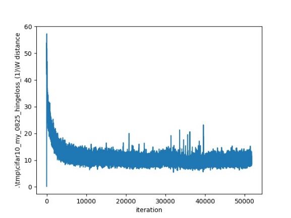
from the original image. In addition, Eq. (2) can be helpful                                 By minimizing the denominator in Eq. (3), the model is
to improve the robustness of the generator, so that it would                              expected to tolerate larger perturbation δ under fixed differ-
not be easily disabled by adversarial noise inputs with slight                            ence  on the i-th pixel. If all pixels of the generated image
perturbations. However, it is difficult to straightforwardly in-                          are simultaneously investigated, we then have
tegrate Eq. (2) into objective function of GANs, because of
the unspecified δ. We next proceed to analyze the appropri-                                             L = min      max       k∇ẑ G(ẑ)kp .        (12)
                                                                                                               G ẑ∈Bp (z,R)
ate δ that satisfies Eq. (2) in the following theorem.
                                                                                             However, maxẑ∈Bp (z,R) k∇ẑ G(ẑ)kp is difficult to calcu-
Theorem 1. Fix  > 0. Given z ∈ Rd as the noise input of
                                                                                          late. Since ẑ lies in a local region around z, it is reasonable
generator Gi , if the perturbation δ ∈ Rd satisfies
                                                                                          to assume that there is a data point ẑ ∼ Pz that can well
                                                                                         approximate ẑ. Hence, we can reformulate Eq. (12) as
            kδkq <                                   ,       (3)
                      maxẑ∈Bp (z,R) k∇ẑ Gi (ẑ)kp
                                                                                                           L = min E k∇z G(z)kp .                    (13)
           1       1                                                                                              G z∼Pz
with       p   +   q   = 1, we have Gi (z + δ) − Gi (z) < .
                                                                                             Though minimizing k∇z G(z)kp will increase the pertur-
Proof. Without loss of generality, we first suppose Gi (z) ≤                              bation δ that can be tolerated by the generator, it is inappro-
Gi (z + δ). Our aim is then to demonstrate what condition δ                               priate to expect an enormously large value of δ, which could
should obey to realize                                                                    damage the diversity of generated images. If the generator is
                         0 ≤ Gi (z + δ) − Gi (z) < .                              (4)    extremely insensitive to changes in the input, linear interpo-
                                                                                          lation in noise space would always lead to the same output.
By the main theorem of calculus, we have                                                  As a result, we introduce a constant number k as a margin to
                          Z 1                                                             constrain the value of k∇z G(z)kp ,
   Gi (z + δ) = Gi (z) +      h∇z Gi (z + tδ), δidt,                               (5)                L = E max(0, k∇z G(z)k2p − k).
                                            0                                                              z∼Pz
                                                                                                                                                     (14)
so that
                                            Z       1
                                                                                          If the value of k∇z G(z)kp is larger than k, there will be
                                                                                          penalty on the generator. Otherwise, we think the value of
 0 ≤ Gi (z + δ) − Gi (z) =                              h∇z Gi (z + tδ), δidt. (6)
                                                0                                         k∇z G(z)kp is sufficient to bring in an appropriate δ for
                                                                                          the generator. This hinge loss is advantageous over classi-
Consider the fact that
 Z 1                                                                                      cal squared loss that expects the gradient magnitude to be
                                                                                          exactly k, as it is unreasonable to set the same gradient mag-
     h∇z Gi (z + tδ), δidt                                                                nitude for data points from distribution Pz .
   0
                                                Z    1
                                                                                   (7)
                                 ≤ kδkq                  k∇z Gi (z + tδ)kp dt,            Smooth GAN
                                                 0                                        So far, we mainly focus on the smoothness of generated im-
where holder inequality is applied and q-norm is dual to the                              ages while neglecting their quality. Considering the genera-
p-norm with p1 + 1q = 1. Suppose that ẑ = z + tδ lies in                                 tion network and the discriminant network within the frame-
a sphere centered at z with a radius R, and we define the                                 work of GANs, we suggest the proposed smooth generator
sphere as Bp (z, R) = {ẑ ∈ Rd | kz − ẑkp ≤ R}. Hence,                                   is beneficial for improving the quality of generated images.
we have                                                                                      Well-trained deep neural networks have been recently
   Z 1                                                                                    found vulnerable to adversarial examples that are impercep-
       k∇z G(z + tδ)kp dt ≤ max k∇ẑ Gi (ẑ)kp . (8)                                      tible to human. Most of the studies on adversarial examples
       0                                        ẑ∈Bp (z,R)                               are for image classification problem. But in image genera-
By combining Eqs. (7) and (8), Eq. (6) can be re-written as                               tion task, we can easily discover failure generations of well-
                                                                                          trained generators as well. The noises resulting in these fail-
  0 ≤ Gi (z + δ) − Gi (z) ≤ kδkq                          max      k∇ẑ Gi (ẑ)kp . (9)   ure cases can thus be regarded as adversarial noise input.
                                                     ẑ∈Bp (z,R)
                                                                                          WGAN-GP (Arjovsky, Chintala, and Bottou 2017) is a re-
 If the right side of Eq. (9) is always upper bounded by ,                               cent promising variant of vanilla GAN,
i.e.,
                       kδkq     max         k∇ẑ Gi (ẑ)kp < ,                   (10)                min E [D(G(z))] − E [D(x)].                    (15)
                              ẑ∈Bp (z,R)                                                               D z∼Pz                  x∼Pd

we can achieve the conclusion that 0 < Gi (z +δ)−Gi (z) <                                 Loss function of WGAN-GP reflects the image quality,
. According to Eq. (10), δ should satisfy                                                which is distinct from loss of vanilla GAN to measure how
                                                                                         well it fools the discriminator. The first term in Eq. (15) is
          kδkq <                                 .    (11)                                relevant to the real sample and has no connection with the
                   maxẑ∈Bp (z,R) k∇ẑ Gi (ẑ)kp
                                                                                          generator. Larger value of D(G(z)) in Eq. (15) therefore in-
By setting z := z + δ and δ := −δ, we we can get the same                                 dicates high quality of generated images. If noise vector z
constraint (i.e., Eq. (11)) over δ to achieve − < Gi (z +                                generates a high-quality image, we expect that its neighbor-
δ) − Gi (z). The proof is completed.                                                      ing point z + δ would generate an image of high quality as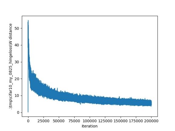
well. To decrease the quality gap between images generated                  Algorithm 1 Smooth GAN
from closed noise inputs, we need to ensure that D(G(z))                    Require: The number of critic iterations per generator iter-
would not drop significantly when the input variates, i.e.,                     ation ncritic , the batch size m, Adam hyperparameters
                                                                                α, β1 , and β2 , the loss balanced coefficient λ, γ.
                        D[G(z + δ)] − D[G(z)] < .                   (16)   Require: initial discriminator parameters w0 , initial gener-
In the following theorem, we analyze what conditions the                        ator parameters θ0 .
perturbation δ should satisfy to guarantee the image quality.                   repeat
                                                                             1: for t = 1, ..., ncritic do
Theorem 2. Fix  > 0. Consider generator G and discrimi-                     2:    for i = 1, ..., m do
nator D in GANs. Given a noise input z ∈ Rd , the generated                  3:       Sample real data x ∼ Pd , latent variable z ∼ Pz , a
image is x̂ = G(ẑ). If the perturbation δ ∈ Rd satisfies                             random number t ∼ U [0, 1].
                                                                            4:       Calculate fake sample Gθ (z), interpolation sample
   kδkq <                                            , (17)                           x̃ ← tx + (1 − t)Gθ (z)
            maxẑ∈Bp (z,R) k∇x̂ D(x̂)kp k∇ẑ G(ẑ)kp
                                                                                                                      (i)
       1       1
                                                                             5:       Calculate the loss function LD ← Dw [Gθ (z)] −
with   p   +   q   = 1, we have D[G(z + δ)] − D[G(z)] < .                            Dw (x) + λ(k∇x̃ D(x̃)k2 − 1)2 ;
                                                                             6:    end for
Proof. Without loss of generality, we first suppose D[G(z +
δ)] ≥ D[G(z)]. Following the proof of Theorem 1, we can                      7:    Update discriminator parameters
                                                                                                       1
                                                                                                          Pm (i)
draw a similar conclusion,                                                         w ← Adam(∇w m             i=1 LD , w, α, β1 , β2 )
                                                                             8: end for
                       0 ≤ D[G(z + δ)] − D[G(z)]
                                                                     (18)    9: Sample a batch of latent variables {z (i) }m  i=1 ∼ Pz .
                         ≤ kδkq max k∇ẑ D[G(ẑ)]kp .                       10: Calculate the loss function
                                 ẑ∈Bp (z,R)
                                                                                  (i)
                                                                                LG ← −Dw [Gθ (z)] + γ max(0, k∇z G(z)k22 − k);
According to the chain rule, we have                                        11: Update generator parameters
                                                                                                   1
                                                                                                      Pm (i)
                       ∇ẑ D[G(ẑ)] = ∇x̂ D(x̂)∇ẑ G(ẑ),            (19)       θ ← Adam(∇θ m            i=1 LG , θ, α, β1 , β2 )
                                                                                until θ has converged
where x̂ = G(ẑ) is the generated image. Given the fact that                Ensure: A smooth generator network G.
  k∇x̂ D(x̂)∇ẑ G(ẑ)kp ≤ k∇x̂ D(x̂)kp k∇ẑ G(ẑ)kp , (20)
where      1
               +   1
                       = 1, Eq. (18) can be re-written as                   where x ∼ PG is the generated sample G(z). Two terms
           p       q
                                                                            k∇x D(x)kp and k∇z G(z)kp are involved in Eq. (25).
       kδkq         max       k∇ẑ D[G(ẑ)]kp                               WGAN-GP (Gulrajani et al. 2017) proposed gradient-
               ẑ∈Bp (z,R)
                                                                     (21)   penalty,
           ≤kδkq             max       k∇x̂ D(x̂)kp k∇ẑ G(ẑ)kp .                     LGP oD = E [(k∇x̃ D(x̃)k2 − 1)2 ],
                         ẑ∈Bp (z,R)
                                                                                                    x̃∼Px
                                                                                                                                     (26)
If the right side of Eq. (21) is always upper bounded by ,                 where Px consists of both real sample distribution Pd and
i.e.                                                                        generated sample distribution PG . By concentrating on gen-
       kδkq            max     k∇x̂ D(x̂)kp k∇ẑ G(ẑ)kp < ,               erated samples x ∼ PG , Eq. (26) encourages k∇x D(x)k2
               ẑ∈Bp (z,R)                                           (22)   to go towards 1, and has been proved to successfully con-
                                                                            strain the norm of the gradient of discriminator k∇x D(x)k2
we then have                                                                in experiments. The remaining term k∇z G(z)kp in Eq. (25)
                                                                           is therefore our only focus. In a similar approach, we en-
  kδkq <                                                    .        (23)
                   maxẑ∈Bp (z,R) k∇x̂ D(x̂)kp k∇ẑ G(ẑ)kp                 courage the norm of the gradient of generator to stay at a
                                                                            lower level and reformulate Eq. (25) to
In the similar approach, we can get the same constraint (i.e.,
Eq. (23)) over δ to achieve − < D[G(z + δ)] − D[G(z)] .                            LGP oG = E max(0, k∇z G(z)k22 − k),              (27)
                                                                                                z∼Pz
The proof is completed.
                                                                            where we set p = q = 2. This equation is exactly the same
  Based on Theorem 2, we propose to minimize                                as Eq. (14).
                                                                               By integrating Eqs. (26) and (27) with WGAN, we obtain
                        max      k∇x̂ D(x̂)kp k∇ẑ G(ẑ)kp ,         (24)   the resulting objective function:
                   ẑ∈Bp (z,R)
                                                                                        L = E [D(G(z))] − E [D(x)]
so that the upper bound over δ will be enlarged and GANs                                     z∼Pz              x∼Pd

model is expect to tolerate more drastic perturbation. Since                              + λ E [(k∇x̃ D(x̃)k2 − 1)2 ]                (28)
it is difficult to discover the optimal ẑ ∈ Bp (z, R), we sup-                               x̃∼Px

pose that there is an approximated ẑ sampled from the dis-                               + γ E max(0, k∇z G(z)k22 − k),
                                                                                              z∼Pz
tribution Pz as well. The loss function can then be reformu-
lated as,                                                                    where λ and γ constant numbers to balance different terms
                                                                            in the function. Our complete algorithm pipeline is summa-
                   min E k∇x D(x)kp k∇z G(z)kp ,                     (25)   rized in Algorithm 1.
                   G,D z∼Pz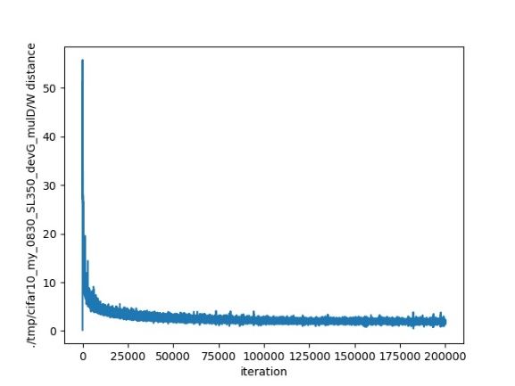
Figure 2: Illustration of image interpolations on the MNIST dataset generated from WGAN-GP (Gulrajani et al. 2017) (left)
and the proposed method (middle and right).

                Experimental Results                                Frechet Inception Distance (FID) (Heusel et al. 2017)
In this section, we conduct comprehensive experiments on a        described the distance between two distributions. FID is
toy dataset and three real-world image datasets, MNIST (Le-       computed as follow:
Cun et al. 1998), CIFAR-10 (Krizhevsky and Hinton 2009),                                                             1

and CelebA (Liu et al. 2015).                                       FID = kµg − µr k22 + Tr(Σg + Σr − 2(Σg Σr ) 2 ),       (29)
                                                                  where (µg , Σg ) and (µr , Σr ) are the mean and covariance of
Datasets and Settings                                             embedded samples from generated distribution Pg and real
In this part, we introduce the real image datasets used in        image distribution Pr , respectively. In the paper, we regard
the experiments and the corresponding experimental settings       the feature maps obtained from a specific layer of the pre-
and network structure. In addition, all the images are nor-       trained Inception model as the embedding of the samples.
malized to pixel values in [−1, +1]. We utilize different net-    FID is more sensitive to the diversity of samples belonging
work architectures on different datasets that was detailed in     to the same category and fixes the drawback of inception
following. The common points are: i) no nonlinear activation      score that is easily fooled by a model which generated only
was attached to the end of discriminators; ii) the minibatch      one image per class. We describe the quality of models to-
used in training process is 64 for both generator and discrim-    gether with the FID and IS score.
inators; iii) Adam optimizer with learning rate 0.0001 and           Multi-scale Structural Similarity for Image Quality
momentum 0.5; iv) noise dimension of 128 for generator; v)        (MS-SSIM) (Wang, Simoncelli, and Bovik 2003) was pro-
weights initialized from Gaussian: N (0; 0.01).                   posed to measuring the similarity of two images. This met-
   MNIST (LeCun et al. 1998) is a handwritten digits              ric well suits to evaluate the quality of samples belonging to
dataset (from 0 to 9) composed of 28 × 28 pixel greyscale         one class. As a result, we apply it to describe the smooth-
images from ten categories. The whole dataset of 70,000 im-       ness of samples obtained from the interpolation opretion. If
ages is split into 60,000 and 10,000 images for training and      two algorithms receive similar FID and IS socores, the sam-
test, respectively. In the experiments on the MNIST dataset,      ples could be equivalent on quality and diversity, and higher
we consider the 10,000 images in test set as valid set in the     MS-SSIM score means a smoother conversion process.
calculation of FID.
   CIFAR-10 (Krizhevsky and Hinton 2009) is a dataset             Interpolation
that consists of 32 × 32 pixel RGB color images drawn from        We implement the images interpolation on the MNIST and
10 categories. There are 60,000 images in the CIFAR-10            CelebA datasets and show a few results in Figures (2) and
dataset which are split into 50,000 training and 10,000 test-     (3). We forward a series of noises obtained by linearly inter-
ing images. We also calculate the FID with 3,000 images           polating between two points in noise space into the model
that was randomly selected in the test set.                       and expect that the resulting images show smooth transposi-
   CelebA (Liu et al. 2015) is a dataset consist of 202,599       tion in the image space.
portraits of celebrities. We use the aligned and cropped ver-        In Figure 2, the left part and the middle part showing the
sion, which preprocesses each image to a size of 64 × 64          similar transposition are generated from models trained with
pixels. 3,000 examples are randomly selected as the test set      WGAN-GP and the Smooth GAN, respectively. The left part
and the rest samples as the training set.                         shows more meaningless images (high lighted in red) during
                                                                  the transposition. When changing an image from one class
Evaluation Metrics                                                to the other one, we want to keep the whole process smooth
We evaluate the proposed method mainly in terms of n three        and meaningful. As shown in the right part of Figure 2, these
metrics well suited to the image domain.                          images accomplish these transpositions by considering im-
   Inception score (IS) (Salimans et al. 2016) rewarding          age qualities and image semantics. For example, the number
high-quality and high-variability of samples, can be ex-          ‘6’ becomes ‘1’ firstly and then becomes ‘9’. Obviously, ‘1’
pressed as: exp(Ex [DKL (p(y|x)kp(y))]), where p(y) =             is more closed to ‘9’ than ‘6’. Interpolation results on the
 1
    PN          i         i
N     i=1 p(y|x = G(z )) is the margin distribution and           other numbers also illustrate this phenomenon. In the results
p(y|x) is the conditional distribution for samples. In this pa-   on the CelebA dataset shown in Figure 3, we achieve great
per, we estimate the IS using a Inception model (Szegedy et       quality while maintaining smoothness, which illustrates the
al. 2016) pretrained in torchvision of PyTorch.                   effectiveness of our approach.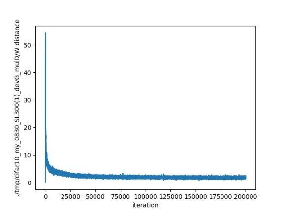
(a) Interpolation images generated from WGAN-GP.

                                        (b) Interpolation images generated from the proposed Smooth GAN.

                                              Figure 3: Image interpolations on the CelebA dataset.

                                                                                                                     46.1
                  DCGAN            WGAN-GP       Smooth GAN
                                                                                         45

                                                         0.827                           40
      24              23.798                                     0.83

                                                                                         35
             23.135

                                                                                   FID
    23.2                                                         0.81                    30                   28.6
                                                 0.797                                        26.3
                                                                                                       24.1
                                                                                         25
    22.4                                                         0.79
                                                                                         20
                               21.831
                                                                                         15
    21.6                                                         0.77
                                                                                              k=100    k=10   k=3    k=0.1
                                         0.755

    20.8                                                         0.75
                                                                                              (a) FID scores                 (b) k = 10
      20                                                         0.73
                       FID                   Sliced MS-SSIM

Figure 4: FID and sliced MS-SSIM obtained by different
models on the CIFAR-10 dataset.

   Taken two images and their interpolation images gener-
ated from the linear interpolations in noise space as a inter-                                       (c) k = 3               (d) k = 0.1
polation slice, to illustrate the effectiveness of the proposed
method in a more convincing way, we generate several slides                    Figure 5: FID scores (a) and Wasserstein distance conver-
on the CelebA dataset. We generated such slices based on                       gence (b, c, d) under different values of k.
different models and calculated the FID and MS-SSIM of
these slices for comparison. Different from calculating the
MS-SSIM score over whole resulting images, we calculated                       exceeds all other models. This is consistent with our obser-
it for every interpolation slice independently. Higher MS-                     vations and demonstrates the effectiveness of our approach.
SSIM values correspond to perceptually more similar im-
ages but also lower diversity and mode collapse (Odena,
Olah, and Shlens 2016; Fedus et al. 2017). Meanwhile,                          Hyperparemeter Analysis To illustrate the choice of the
higher FID score ensures the diversity and prevents the                        value of k, we show FID scores and Wasserstein distance
GANs from mode collapse. As a result, considering together                     convergence curves of experiments with different k values
with FID, the MS-SSIM score could focus on indicating the                      on the CIFAR-10 dataset in Figure 5. Figure 5 (a) shows
similarity of images, which is consistent with smooth trans-                   the FID scores obtained from four k values, and K = 10
position in an interpolation slide. The sliced MS-SSIM score                   provides the best score. Figure 5 (b) shows that the experi-
used in this experiment can be described as:                                   ment with k = 10 achieves the best convergence. Setting k
                N −1 N
                                                                               to 3 will influence the training progress and achieve slightly
      N (N − 1) X X                                                            higher Wasserstein distance than Figure 5 (b) when network
                          MS − SSIM(Si , Sj ),                          (30)
          2                                                                    convergence. The generator is failed to produce enough real-
                i=1 j=i+1
                                                                               istic images when setting k to 0.1; this is because too small
where Si is the i-th slide of samples in the resulting group.                  a k value will suppress the diversity of generator output.
Now, we could estimate the effectiveness with FID and                          Moreover, a large value of k relaxes the constraint on the
sliced MS-SSIM. We report the FID and sliced MS-SSIM                           gradient and can result in insufficient smoothness of the net-
obtained on the CelebA dataset in Figure 4. Our model not                      work output. In our experiments, we used different k values
only has the lowest FID score, but also its MS-SSIM score                      based on experimental results regarding different datasets.
Figure 6: Samples generated from the proposed model trained on MNIST (left), CIFAR-10 (middle), and CelebA (right).

50                                                   44
                                                                                                                                                                             DCGAN
40                                                                                                             36                                                            WGAN-GP
                                                                  32
                                                                         29
                                                                                    27          27                              27                                           Smooth GAN
30                                  24                                                               25

20                                                                                         15
                                                                              12
                                              10                                                                     10
                             7                                                                                                                   8
10                                                           6                                                                        6
                    3                                                                                     2                 3                                    2
        0    1          0                1                                                                                                   0        1      0        1      0   1    0      0
 0
            45-46           46-47            47-48               48-49             49-50          50-51             51-52            52-53           53-54           54-55           55-56
                                                                                                 FID

                                                          Figure 7: FID distribution obtained on several subsets.

                                                                                                          uate the quality of the generated samples. However, FID
Table 1: Incetion scores (higher is better) and FIDs (lower is                                            only provides an average quality of the whole test images.
better) on the CIFAR-10 dataset.                                                                          First, we generate a sufficient large set of images (50,000
                 Method                                                IS ↑          FID ↓
                                                                                                          in experiments). Next, we randomly sample 512 images to
                 DCGAN
                                                                 6.40 ± .05              36.7             form a subset and calculate the FID of this subset. We repeat
   (Radford, Metz, and Chintala 2015)
                 BEGAN                                                                                    the second step 120 times and calculate their FID scores.
                                                                 5.62 ± .07              32.3             By comparing these FIDs obtained from subsets, we can
  (Berthelot, Schumm, and Metz 2017b)
                 WGAN                                                                                     roughly estimate the quality distribution of the samples. Fig-
                                                                 3.82 ± .06              42.8
  (Arjovsky, Chintala, and Bottou 2017)                                                                   ure 7 shows the distribution of FID scores calculated over
      D2GAN (Nguyen et al. 2017)                               7.15 ± .07             30.6                subsets and obtained from three models. Compared to other
    WGAN-GP (Gulrajani et al. 2017)                            7.36 ± .07             26.5                models, our model can obtain lower FID scores, while big-
          Smooth GAN (Ours)                                   7.66 ± .05              24.1                ger value of FIDs are less. Moreover, the FID scores ob-
                                                                                                          tained from the proposed model are mainly concentrated be-
                                                                                                          tween 46 and 50, and only 8 scores of subset fall outside
Image Generation                                                                                          this region, while the other two algorithms get a loose distri-
We conduct experiments on three real image datasets to in-                                                bution of FID scores. Therefore, our method can effectively
vestigate the capabilities of the proposed method. Table 1 re-                                            reduce the low-quality samples in the generated samples.
ports the inception scores and FIDs on the CIFAR-10 dataset
which obtained from the proposed model and baseline meth-                                                                                 Conclusions
ods. In this results, the proposed method outperforms almost
state-of-the-art methods. Therefore, the proposed method                                                  Here we analyze the relationship between perturbation on
provides considerable quality on the three datasets.                                                      the input of the generator and its influence on the output im-
   Figure 6 shows several samples generated by the model                                                  ages. By investigating the tolerable input perturbation, we
learned with the proposed method. The samples on the                                                      develop a smooth generator. We further integrate this smooth
MNIST dataset show a variety of numbers and styles. Dogs,                                                 generator with a gradient penalized discriminator, and pro-
trucks, boats, and fish could also be found in the samples on                                             duce smooth GAN that generate stable and high-quality im-
the CIFAR-10 dataset. Age and gender diversity can also be                                                ages. Experiments on real-world image datasets demonstrate
observed in the results on the CelebA dataset. These results                                              the necessity of studying smooth generator and show the
confirm the capabilities of the proposed method.                                                          proposed method is capable of learning smooth GAN.

Samples Quality Distribution                                                                                                     Acknowledgments
In this section, we introduce a way to describe the quality                                               We thank supports of the NSFC under Grant 61876007 and
distribution of samples and demonstrate the effectiveness of                                              61872012, ARC Projects FL-170100117, DP-180103424,
the proposed method that can effectively reduce the num-                                                  IH-180100002, DE-180101438, and Beijing Major Science
ber of low-quality images. FID is a good indicator to eval-                                               and Technology Project Z171100000117008.
References Gradient-based learning applied to document recognition.
Arjovsky, M.; Chintala, S.; and Bottou, L. 2017. Wasserstein Proceedings of the IEEE 86(11):2278–2324.
gan. arXiv preprint arXiv:1701.07875. Li, C.; Xu, K.; Zhu, J.; and Zhang, B. 2017a. Triple genera-
tive adversarial nets. arXiv preprint arXiv:1703.02291.
Berthelot, D.; Schumm, T.; and Metz, L. 2017a. Be-
gan: boundary equilibrium generative adversarial networks. Li, C.-L.; Chang, W.-C.; Cheng, Y.; Yang, Y.; and Póczos,
arXiv preprint arXiv:1703.10717. B. 2017b. Mmd gan: Towards deeper understanding of mo-
ment matching network. In Advances in Neural Information
Berthelot, D.; Schumm, T.; and Metz, L. 2017b. BE-
Processing Systems, 2203–2213.
GAN: boundary equilibrium generative adversarial net-
works. CoRR abs/1703.10717. Liu, Z.; Luo, P.; Wang, X.; and Tang, X. 2015. Deep learn-
ing face attributes in the wild. In Proceedings of the IEEE
Bojanowski, P.; Joulin, A.; Lopez-Paz, D.; and Szlam, A. International Conference on Computer Vision, 3730–3738.
2017. Optimizing the latent space of generative networks.
arXiv preprint arXiv:1707.05776. Makhzani, A.; Shlens, J.; Jaitly, N.; Goodfellow, I.; and
Frey, B. 2015. Adversarial autoencoders. arXiv preprint
Chen, X.; Duan, Y.; Houthooft, R.; Schulman, J.; Sutskever, arXiv:1511.05644.
I.; and Abbeel, P. 2016. Infogan: Interpretable representa-
tion learning by information maximizing generative adver- Mao, X.; Li, Q.; Xie, H.; Lau, R. Y.; Wang, Z.; and Smolley,
sarial nets. In Advances in neural information processing S. P. 2017. Least squares generative adversarial networks.
systems, 2172–2180. In Computer Vision (ICCV), 2017 IEEE International Con-
ference on, 2813–2821. IEEE.
Chen, X.; Xu, C.; Yang, X.; and Tao, D. 2018. Attention-gan
for object transfiguration in wild images. In The European Mirza, M., and Osindero, S. 2014. Conditional generative
Conference on Computer Vision (ECCV). adversarial nets. arXiv preprint arXiv:1411.1784.
Chen, X.; Xu, C.; Yang, X.; Song, L.; and Tao, D. 2019. Nguyen, T.; Le, T.; Vu, H.; and Phung, D. 2017. Dual dis-
Gated-gan: Adversarial gated networks for multi-collection criminator generative adversarial nets. In Advances in Neu-
style transfer. IEEE Transactions on Image Processing ral Information Processing Systems, 2670–2680.
28(2):546–560. Odena, A.; Olah, C.; and Shlens, J. 2016. Conditional im-
age synthesis with auxiliary classifier gans. arXiv preprint
Denton, E. L.; Chintala, S.; Szlam, A.; and Fergus, R. 2015.
arXiv:1610.09585.
Deep generative image models using a laplacian pyramid of
adversarial networks. CoRR abs/1506.05751. Radford, A.; Metz, L.; and Chintala, S. 2015. Unsupervised
representation learning with deep convolutional generative
Fedus, W.; Rosca, M.; Lakshminarayanan, B.; Dai, A. M.;
adversarial networks. arXiv preprint arXiv:1511.06434.
Mohamed, S.; and Goodfellow, I. 2017. Many paths to equi-
librium: Gans do not need to decrease adivergence at every Salimans, T.; Goodfellow, I.; Zaremba, W.; Cheung, V.; Rad-
step. arXiv preprint arXiv:1710.08446. ford, A.; and Chen, X. 2016. Improved techniques for train-
ing gans. In Advances in Neural Information Processing
Goodfellow, I.; Pouget-Abadie, J.; Mirza, M.; Xu, B.; Systems, 2234–2242.
Warde-Farley, D.; Ozair, S.; Courville, A.; and Bengio, Y.
2014. Generative adversarial nets. In Advances in neural Szegedy, C.; Vanhoucke, V.; Ioffe, S.; Shlens, J.; and Wojna,
information processing systems, 2672–2680. Z. 2016. Rethinking the inception architecture for computer
vision. In Proceedings of the IEEE conference on computer
Gulrajani, I.; Ahmed, F.; Arjovsky, M.; Dumoulin, V.; and vision and pattern recognition, 2818–2826.
Courville, A. C. 2017. Improved training of wasserstein
gans. In Advances in Neural Information Processing Sys- van den Oord, A.; Kalchbrenner, N.; Espeholt, L.; Vinyals,
tems, 5767–5777. O.; Graves, A.; et al. 2016. Conditional image generation
with pixelcnn decoders. In Advances in Neural Information
Heusel, M.; Ramsauer, H.; Unterthiner, T.; Nessler, B.; Processing Systems, 4790–4798.
Klambauer, G.; and Hochreiter, S. 2017. Gans trained by
a two time-scale update rule converge to a nash equilibrium. Wang, Z.; Simoncelli, E. P.; and Bovik, A. C. 2003. Multi-
arXiv preprint arXiv:1706.08500. scale structural similarity for image quality assessment. In
The Thrity-Seventh Asilomar Conference on Signals, Sys-
Karras, T.; Aila, T.; Laine, S.; and Lehtinen, J. 2017. Pro- tems & Computers, 2003, volume 2, 1398–1402. Ieee.
gressive growing of gans for improved quality, stability, and
Zhai, S.; Cheng, Y.; Feris, R.; and Zhang, Z. 2016. Gener-
variation. arXiv preprint arXiv:1710.10196.
ative adversarial networks as variational training of energy
Kim, T., and Bengio, Y. 2016. Deep directed genera- based models. arXiv preprint arXiv:1611.01799.
tive models with energy-based probability estimation. arXiv
preprint arXiv:1606.03439.
Kingma, D. P., and Welling, M. 2013. Auto-encoding vari-
ational bayes. arXiv preprint arXiv:1312.6114.
Krizhevsky, A., and Hinton, G. 2009. Learning multiple
layers of features from tiny images.
LeCun, Y.; Bottou, L.; Bengio, Y.; and Haffner, P. 1998.You can also read