A Three-Way Model for Collective Learning on Multi-Relational Data
←
→
Page content transcription
If your browser does not render page correctly, please read the page content below
A Three-Way Model for Collective Learning on Multi-Relational Data

Maximilian Nickel                                                                                NICKEL @ CIP. IFI . LMU . DE
Ludwig-Maximilians-Universität, Munich, Germany
Volker Tresp                                                                              VOLKER . TRESP @ SIEMENS . COM
Siemens AG, Corporate Technology, Munich, Germany
Hans-Peter Kriegel                                                                             KRIEGEL @ DBS . IFI . LMU . DE
Ludwig-Maximilians-Universität, Munich, Germany

                         Abstract                                tensors in this domain is manifold. From a modelling per-
                                                                 spective tensors provide simplicity, as multiple relations of
     Relational learning is becoming increasingly im-
                                                                 any order can be expressed straightforwardly as a higher-
     portant in many areas of application. Here, we
                                                                 order tensor. Moreover, no a priori knowledge about the
     present a novel approach to relational learning
                                                                 structure of the problem needs to be known or needs to be
     based on the factorization of a three-way tensor.
                                                                 inferred from the data, as it is necessary e.g. for graphical
     We show that unlike other tensor approaches, our
                                                                 models like Bayesian Networks or Markov Logic Networks
     method is able to perform collective learning via
                                                                 (MLN). A reason to employ tensor decompositions from a
     the latent components of the model and provide
                                                                 learning perspective is that relational domains are usually
     an efficient algorithm to compute the factoriza-
                                                                 high-dimensional and sparse, a setting where factorization
     tion. We substantiate our theoretical considera-
                                                                 methods have shown very good results.
     tions regarding the collective learning capabili-
     ties of our model by the means of experiments on            An important property of relational data is that correlations
     both a new dataset and a dataset commonly used              can be produced between multiple interconnected nodes.
     in entity resolution. Furthermore, we show on               These correlations can be captured by including the at-
     common benchmark datasets that our approach                 tributes, relations or classes of related entities in a learning
     achieves better or on-par results, if compared to           task. However, well-known tensor factorization approaches
     current state-of-the-art relational learning solu-          such as CANDECOMP/PARAFAC (CP) (Harshman &
     tions, while it is significantly faster to compute.         Lundy, 1994) or Tucker (Tucker, 1966) cannot model this
                                                                 collective learning effect sufficiently. The DEDICOM de-
                                                                 composition (Harshman, 1978) is capable of detecting this
1. Introduction                                                  type of correlations, but unfortunately, it puts constraints
                                                                 on the model that are not reasonable for relational learning
With the growing relevance of relational data and network        in general and thus leads to suboptimal results. In this pa-
data in such diverse areas as social network modeling, the       per we propose the relational learning approach RESCAL
semantic web, bioinformatics and artificial intelligence, the    which is based on a tensor factorization that is related to
field of relational learning is increasing in importance. This   DEDICOM but does not exhibit the same constraints. In
paper is concerned with the application of tensors to re-        doing so we are able to derive models of higher quality and
lational learning. Tensors and their decompositions are          with significant runtime improvements. We will present
widely used in fields like psycho- or chemometrics and           an efficient algorithm for computing the factorization and
more recently have also been applied to data mining and          evaluate our approach on both a new collective learning
machine learning problems, e.g. for modelling temporal ef-       dataset and relational learning benchmark datasets. We
fects in social networks. In relational learning, tensors have   will show that significant improvements can be achieved
just emerged to be used as an alternative to more common         by using our model compared to more commonly used ten-
approaches like graphical models. The motivation to use          sor models like CP. Furthermore, we will also show that
                                                                 our approach gives better or similar results if compared to
Appearing in Proceedings of the 28 th International Conference
                                                                 current state-of-the-art approaches in relational learning on
on Machine Learning, Bellevue, WA, USA, 2011. Copyright 2011
by the author(s)/owner(s).                                       these datasets, while only taking a fraction of the time to
A Three-Way Model for Collective Learning on Multi-Relational Data
compute. et al., 2006) are nonparametric Bayesian approaches to
relational learning, while (Singh & Gordon, 2008) em-
2. Modelling and Notation ploy collective matrix factorizations for relational learn-
ing. (Getoor & Taskar, 2007) presents further approaches
The modelling approach of relational domains in this pa- and gives a detailed introduction into the area of relational
per is the following. To represent dyadic relational data learning. Tensor decompositions have been widely applied
we make use of the semantic web’s RDF formalism where to fields like psycho- and chemometrics. An extensive re-
relations are modeled as triples of the form (subject, view of tensor decompositions and their applications can
predicate, object) and where a predicate either be found in (Kolda & Bader, 2009). Recently, (Sutskever
models the relationship between two entities or between et al., 2009) introduced the Bayesian Clustered Tensor Fac-
an entity and an attribute value. In order to model dyadic torization (BCTF) and applied it to relational data. (Sun
relational data as a tensor, we employ a three-way tensor et al., 2006) presents methods for dynamic and streaming
X , where two modes are identically formed by the concate- tensor analysis. These methods are used to analyse network
nated entities of the domain and the third mode holds the re- traffic and bibliographic data. (Franz et al., 2009) use CP
lations.1 Figure 1 provides an illustration of this modelling to rank relational data that is given in form of RDF triples.
method. A tensor entry Xijk = 1 denotes the fact that there
exists a relation (i-th entity, k-th predicate, 4. Methods and Theoretical Aspects
j-th entity). Otherwise, for non-existing and un-
known relations, the entry is set to zero. Relational learning is concerned with domains where enti-
ties are interconnected by multiple relations. Hence, corre-
lations can not only occur directly between entities or re-
lations, but also across these interconnections of different
entities and relations. Depending on the learning task at
hand, it is known that it can be of great benefit when the
learning algorithm is able to detect these relational learn-
ing specific correlations reliably. For instance, consider the
task of predicting the party membership of a president of
the United States of America. Without any additional infor-
mation, this can be done quite accurately when the party of
Figure 1: Tensor model for relational data. E1 · · · En denote the the president’s vice president is known, since both persons
entities, while R1 · · · Rm denote the relations in the domain
have mostly been members of the same party. To include
information such as attributes, classes or relations of con-
In the remainder of this paper we will use the following nected entities to support a classification task is commonly
notation: Tensors are represented by calligraphic letters X , referred to as collective classification. However, this proce-
while Xk refers to the k-th frontal slice of the tensor X . dure can not only be useful in classification problems, but
X(n) denotes the unfolding of the tensor X in mode n. A ⊗ also in entity resolution, link prediction or any other learn-
B refers to the Kronecker product of the matrices A and B. ing task on relational data. We will refer to the mechanism
Ik denotes the identity matrix of size k and vec(X) is the of exploiting the information provided by related entities
vectorization of the matrix X. Vectors are represented by regardless of the particular learning task at hand as collec-
bold lowercase letters, e.g. a. Furthermore, it is assumed tive learning.
that the data is given as a n × n × m tensor X , where n is
the number of entities and m the number of relations. 4.1. A Model for Multi-Relational Data
To perform collective learning on multi-relational data, we
3. Related Work propose RESCAL, an approach which uses a tensor factor-
ization model that takes the inherent structure of relational
The literature on statistical relational learning is vast, thus
data into account. More precisely, we employ the follow-
we will only give a very brief overview. A common ap-
ing rank-r factorization, where each slice Xk is factorized
proach to relational learning is to employ graphical mod-
as
els such as Bayesian Networks or Markov Logic net-
works (Friedman et al., 1999; Richardson & Domingos, Xk ≈ ARk AT , for k = 1, . . . , m (1)
2006). Moreover, IHRM (Xu et al., 2006) and IRM (Kemp
1
Please note that we don’t assume homogeneous domains, Here, A is a n×r matrix that contains the latent-component
thus the entities of one mode can be instances of multiple classes representation of the entities in the domain and Rk is an
like persons, items, places, etc. asymmetric r × r matrix that models the interactions of theA Three-Way Model for Collective Learning on Multi-Relational Data
latent components in the k-th predicate.
Bill John
The factor matrices A and Rk can be computed by solving
party party
the regularized minimization problem
min f (A, Rk ) + g(A, Rk ) (2) vicePresidentOf Party X vicePresidentOf
A,Rk
where party party
! Al Lyndon
1 X
f (A, Rk ) = kXk − ARk AT k2F (3)
2
k
Figure 2: Visualization of a subgraph of the relational graph for
and g is the following regularization term the US presidents example. The relation marked red is unknown.
!
1 X
g(A, Rk ) = λ kAk2F + kRk k2F (4)
2 aTJohn Rparty aPartyX and as such the missing relation can be
k
predicted correctly. Please note that this information prop-
which is included to prevent overfitting of the model. agation mechanism through the latent components would
break if Bill and John would have different representa-
An important aspect of (1) for collective learning and what
tions as subjects and objects.
distinguishes it from other tensor factorizations like CP or
even BCTF is that the entities of the domain have a unique
latent-component representation, regardless of their occur- 4.2. Connections to other Tensor Factorizations
rence as subjects or objects in a relation, as they are repre- The model specified in (1) can be considered a relaxed
sented both times by the matrix A. The effect of this mod- version of DEDICOM or equivalently, an asymmetric ex-
elling becomes more apparent by looking at the element- tension of IDIOSCAL. The rank-r DEDICOM decom-
wise formulation of (3), namely position of a three-way tensor X is given as: Xk ≈
ADk RDk AT , for k = 1, . . . , m. Here, A is a n×r matrix
1X 2
f (A, Rk ) = Xijk − aTi Rk aj that contains the latent components and R is an asymmetric
2
i,j,k r × r matrix that models the global interactions of the la-
tent components. The diagonal r × r matrix Dk models the
Here, ai and aj denote the i-th and j-th row of A and participation of the latent components in the k-th predicate.
thus are the latent-component representations of the i- Thus, DEDICOM is suitable when there is one global in-
th and j-th entity. By holding aj and Rk fixed, it teraction model for the latent components and its variation
is clear that the latent-component representation ai de- across the third mode can be described by diagonal factors.
pends on aj as well as the existence of the triple (i-th Examples where this is a reasonable assumption include
entity, k-th predicate, j-th entity) repre- international trade or communication patterns across time,
sented by Xijk . Moreover, since the entities have a unique as presented in (Bader et al., 2007). However, for multi-
latent-component representation, aj holds also the infor- relational data this assumption is often too restricted.
mation which entities are related to the j-th entity as sub-
jects and objects. Consequently, all direct and indirect re- Furthermore, the model (1) can be regarded as a restricted
lations have a determining influence on the calculation of Tucker3 model. Let X(n) = AG(n) (C ⊗ B)T be the matri-
ai . Just as the entities are represented by A, each relation is cized form of the Tucker3 decomposition of X . (1) is then
represented by the matrix Rk , which models how the latent equivalent to a Tucker3 model, where the factors B and C
components interact in the respective relation and where are constrained to B = A and C = Ik , while G is holding
the asymmetry of Rk takes into account whether a latent the slices Rk .
component occurs as a subject or an object.
4.3. Computing the Factorization
For a short illustration of this mechanism, consider the
example shown in Figure 2. The latent-component rep- In order to compute the factor matrices for (1), equation (2)
resentations of Al and Lyndon will be similar to each could be solved directly with any nonlinear optimization
other in this example, as both representations reflect that algorithm. However, to improve computational efficiency
their corresponding entities are related to the object Party we take an alternating least-squares (ALS) approach and
X. Because of this, Bill and John will also have sim- exploit the connection of (1) to DEDICOM, by using the
ilar latent-component representations. Consequently, the very efficient ASALSAN (Bader et al., 2007) algorithm as
product aTBill Rparty aPartyX will yield a similar value to a starting point and adapting it to our model. In particular,A Three-Way Model for Collective Learning on Multi-Relational Data
we employ the following algorithm: Rk such that A and Xk are only r × r matrices. In do-
ing so, updating Rk becomes independent from the num-
Update A: To compute the update step of A we use
ber of entities and is only dependent on the complexity of
the same approach as ASALSAN and solve the problem
the model. Despite its similarities to DEDICOM, there are
approximately for left and right A simultaneously for all
significant computational advantages of our approach, as a
frontal slices of X . The data is stacked side by side for
simpler model is computed. Evidently, (1) has no Dk fac-
this, such that
tors, a problem that has to be solved in ASALSAN by New-
−1
X̄ = AR̄(I2m ⊗ AT ) (5) ton’s method. Moreover, in RESCAL the term Z T Z Z
isn’t dependent on k and thus only needs to be computed
where once beforeupdating all Rk . Computing the inverse of
Z T Z + λI is the most expensive operation in updating
X̄ = (X1 X1T . . . Xm Xm
T
) Rk , as Z is the result of a Kronecker product and thus can
R̄ = (R1 R1T . . . Rm Rm
T
) become very large. However, in case Rk is not regularized,
this can be simplified. Since (A⊗B)(C ⊗D) = AC ⊗BD
We approximate this nonlinear problem by solving only for and (A ⊗ B)−1 = (A−1 ⊗ B −1 ) (Horn & Johnson, 1994)
the left A while holding the right A constant. As (Bader it holds that
et al., 2007) points out, this approach seems to be viable −1 −1 −1
because of the construction of X̄. Let Ā denote the constant ZT Z = AT A A ⊗ AT A A
right hand A. Then, the gradient of (5) is given by
Here, the inverse only has to be computed for the much
∂f smaller matrix AT A. Furthermore, since m occurs only
= R̄[(I ⊗ ĀT Ā)R̄T AT − (I ⊗ ĀT )X̄ T ] + λAT as a linear factor, the algorithm will scale linearly with
∂A
the number of predicates. But the simplicity of the model
By using the method of normal equations and setting this comes also at a cost. It can be seen from (1) and the rep-
gradient to zero, the update of A can be computed by resentation as a Tucker3 model that no rank reduction is
" #" #−1 performed on the mode that holds the relations, what po-
m m
X X tentially can have a negative effect when the relations are
A← Xk ARkT + XkT ARk Bk + Ck + λI
noisy and should be aggregated simultaneously with the en-
k=1 k=1
tities.
where
4.4. Solving Relational Learning Tasks
Bk = Rk AT ARkT , Ck = RkT AT ARk
Canonical relational learning tasks can be approached with
Update Rk : By holding A fixed and vectorizing Xk as RESCAL in the following way. To predict whether a link
well as Rk , the minimization problem (3) can be cast as exists between two entities ei , ej for the k-th predicate,
it is sufficient to look at the rank-reduced reconstruction
f (Rk ) = kvec(Xk ) − (A ⊗ A)vec(Rk )k X̂k = ARk AT of the appropriate slice Xk . In doing so,
+λkvec(Rk )k link prediction can be done by comparing X̂ijk > θ to
some given threshold θ or by ranking the entries accord-
what is a regularized linear regression problem and can be ing to their likelihood that the link in question exists.
solved accordingly, i.e. by
Collective classification can be cast as a subtask of link pre-
T
−1 diction, as the class of an entity can be modelled by intro-
Rk ← Z Z + λI Zvec(Xk )
ducing a class relation and including the classes as entities
where Z = A ⊗ A. in the tensor. Thus, the classification problem can also be
solved by reconstructing the appropriate slice of the class
The starting points for A and Rk can either be random ma- relation. The collectivity of the classification, as for all
P or A isTinitialized from the eigendecomposition of
trices other learning tasks, is given automatically by the structure
k (Xk + Xk ). To compute the factor matrices, the al- of the model.
gorithm performs alternating updates of A and all Rk until
f (A,Rk )
converges to some small threshold or a maximum Furthermore, the matrix A can be regarded as the entity-
kX k2F
latent-component space that is created by the decomposi-
number of iterations is exceeded.
tion. Link-based clustering can be performed by clustering
One benefit of RESCAL is that it can be computed effi- the entities in this entity-latent-component space. In doing
ciently. Similar to the ASALSAN algorithm, it is possible so, the similarity between entities is computed upon their
to use the QR decomposition of A and Xk for updating similarity across multiple relations.A Three-Way Model for Collective Learning on Multi-Relational Data
Prediction of party membership
1.0
0.8 0.74 0.78
0.64
AUC
0.6
0.44 0.48
0.4
0.2 0.16
0.0
om CP S G L
nd C OM UN +A CA
Ra DI S NS RES
DE SU
(a) (b)
Figure 3: (a) is a visualization of the presidentOf relation on the US presidents dataset. The size of the ring segments indicates
how many persons in the dataset are members of the respective party. An arc indicates a presidentOf relation and the size of an arc
indicates how often this relation occurs between the connected segments. (b) shows the results of 10-fold cross-validation on this data.
5. Evaluation factorizations CP and DEDICOM. Moreover, we included
the SUNS algorithm (Huang et al., 2010) in the evaluation,
In the following we evaluate RESCAL in comparison to a relational learning approach for large scale data. Despite
standard tensor factorizations and relational learning algo- SUNS’ ability to handle large data sizes, its capabilities
rithms on various datasets. All algorithms have been im- for collective learning are limited. Therefore, SUNS is a
plemented in Python and evaluated on a Intel Core 2 Duo good indicator what improvement can be gained in collec-
2.5GHz with 4GB RAM. For CP we implemented the CP- tive learning. For the same reason we included Aggregated
ALS algorithm of the Tensor Toolbox (Bader & Kolda, SUNS (SUNS+AG), which mimics collective learning and
2010) in Python/NumPy. thus is the counterpart of SUNS without aggregation.3 To
evaluate the algorithms we’ve conducted cross-validation
5.1. Collective Classification by partitioning all persons into ten folds and deleting the
The first experiment in this evaluation is designed to as- party membership information of the persons in the test
sess, in a controlled setting, the collective learning capa- fold. In the case of RESCAL, CP and DEDICOM we com-
bilities of our approach as discussed in Section 4. For puted a rank-reduced factorization, ranked all parties by
this purpose, we created a dataset for the US presi- their entries in the reconstructed party-membership-slice
dents example, by retrieving the names of all presidents and recorded the area under the precision-recall curve. It
and vice presidents of the United States from DBpe- can be seen from Figure 3(b) that aggregation improves
dia, in combination with their party membership and the the SUNS model significantly. The results of RESCAL
presidentOf/vicePresidentOf information.2 The and DEDICOM outperform both CP and SUNS and show
objective of the experiment is to predict the party mem- clearly the usefulness of our approach for domains where
bership for each person in a collective classification set- collective learning is an important feature. It can also be
ting. It can be seen from Figure 3(a), that a president and seen that CP isn’t capable of collective learning, as it yields
his/her vice president have mostly been members of the similar results to SUNS. There is also a significant differ-
same party. Hence, the ability to perform collective learn- ence between the results of RESCAL and DEDICOM, what
ing by including the party of a related person should greatly indicates that, even on this small dataset with highly corre-
improve the classification results, especially as the dataset lated predicates, the constraints imposed by DEDICOM are
contains no further information other than the three rela- to restrictive.
tions that could help in predicting the correct party. From
the raw RDF data we constructed a 93 × 93 × 3 tensor, 5.2. Collective Entity Resolution
where the entity modes correspond to the joint set of per- The US presidents example demonstrated the capabilities
sons and parties and the third mode is formed by the three of our approach on a small, specially created dataset. In
relations. In addition to RESCAL we evaluated the tensor
3
2 Here, aggregation means that the party membership informa-
Dataset available at
tion of the related person has been added manually as a new rela-
http://www.cip.ifi.lmu.de/~nickel
tion to each statistical unitA Three-Way Model for Collective Learning on Multi-Relational Data
Cora - Citations Cora - Author Cora - Venue
0.988 0.987 0.992 0.970
Venue 1.0 0.915 1.0 1.0 0.911
0.886 0.896
0.807
0.8 0.8 0.8 0.736
Title 0.601
AUC
AUC
AUC
Citation 0.6 0.6 0.6
0.4 0.4 0.4 0.387
0.2 0.2 0.2
Author
0.0 0.0 0.0
) ) ) ) B) )
(B TS CP CA
L (B TS CP AL N( TS CP AL
N C
ES
N C SC BC SC
ML N (B R ML N (B RE ML N( RE
ML ML ML
(a) (b) (c) (d)
Figure 4: (a) shows the structural representation of the Cora dataset. (b)-(d) show the results for the area under the precision-recall
curve for 5-fold entity resolution runs on this dataset
turn, the Cora dataset is a larger real-world dataset which at directly connected entities in order to perform entity
is commonly used to assess the performance of relational resolution for citations. But the citations are noisy them-
learning approaches in tasks like collective classification or selves. Therefore, when entity resolution has to be done
entity resolution. It is especially interesting as it is known for an author or a venue, it is very helpful for an algorithm
that applying collective learning to this dataset can improve when it can include the entities that are connected to an
the quality of the model significantly (Sen et al., 2008). author’s or venue’s citation in its evaluation of the entity.
Cora exists in different versions, here we use the dataset This circumstance is reflected in the evaluation results in
and experimental setup as described in (Singla & Domin- Figure 4. For citations there is no significant difference be-
gos, 2007) and also compare our results to those reported in tween RESCAL and CP. For authors and venues however,
that publication. From the raw data we constructed a tensor RESCAL gives far better results than CP, as it can perform
of size 2497 × 2497 × 7. collective learning. In the case of venues, it shows even
better results than the much more complex MLN.
The objective of this experiment is to perform entity reso-
lution, as described in the following: While MLNs have to
treat entity resolution as a link prediction problem, i.e. by 5.3. Kinships, Nations and UMLS
predicting the probability of the triple (x, isEqual, In order to evaluate how well RESCAL is performing com-
y), tensor factorizations allow us take a different approach. pared to current state-of-the-art relational learning solu-
We derive the likelihood that two entities are identical tions, we applied it to the Kinships, Nations and UMLS
from their similarity in the entity-latent-component space datasets used in (Kemp et al., 2006) and compared the area
A. More specifically, we normalize the rows of A, such that under the precision-recall curve (AUC) to the results of
each row represents the normalized participation of the cor- BCTF, IRM and MRC published in (Sutskever et al., 2009)
responding entity in the latent components. Based on this and (Kok & Domingos, 2007). Due to space constraints we
representation we compute the similarity between two en- refer to (Kemp et al., 2006) for a detailed description of the
2
tities x, y by using the heat kernel k(x, y) = e−kx−yk /δ , datasets. In order to get comparable results to BCTF, IRM
where δ is a user-given constant and use this similarity and MRC we followed their experimental protocol and
score as a measure for the likelihood that x and y refer performed 10-fold cross-validation by using (subject,
to the same entity. This is a relative ad hoc approach to predicate, object) triples as the statistical unit. For
entity resolution, but the focus of this experiment is again a comparison to standard tensor decompositions we’ve in-
rather on assessing the collective learning capabilities of cluded CP and DEDICOM in the evaluation. The task for
our approach than conducting a full entity resolution ex- all three datasets is link prediction. Figure 5 shows the re-
periment. We are mainly interested whether our approach sults of our evaluation. It can be seen that RESCAL gives
can produce results roughly similar to MLNs and how they comparable or better results than BCTF, IRM and MRC on
compare to CP. Figure 4 shows the results of our evalua- all datasets.
tion, which are especially interesting in combination with
At last we want to briefly demonstrate the link-based clus-
the structural representation of the data. Since the Cita-
tering capabilities of RESCAL. Therefore, we computed a
tion class is the central node in Figure 4 and the other
rank-20 decomposition of the Nations dataset and applied
classes aren’t interconnected, it is sufficient to look onlyA Three-Way Model for Collective Learning on Multi-Relational Data
Kinships UMLS Nations
0.95 0.98 0.98 0.98
1.0 0.94 0.90 1.0 0.95 0.95 1.0
0.85 0.83 0.81 0.84
0.8 0.75 0.75
0.8
0.69 0.66
0.8 0.70
AUC
AUC
AUC
0.6 0.6 0.6
0.4 0.4 0.4
0.2 0.2 0.2
0.0 0.0 0.0
CP OM T
F M
MR
C
CA
L CP OM T
F M
MR
C AL CP M M C AL
IC BC IR
ES IC BC IR SC CO IR MR SC
D R D RE DI RE
DE DE DE
Figure 5: Link prediction results for the Kinships, Nations and UMLS datasets
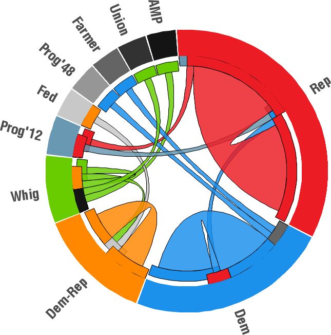
k-means with k = 6 to the matrix A. It can be seen from reasons. The simpler model of RESCAL allows significant
Figure 6 that in doing so, similar clusters as in (Kemp et al., improvements with regard to the computational complex-
2006) are obtained. The countries are partitioned into one ity, as discussed in Section 4. But interestingly, RESCAL
group containing countries from the communist bloc, two shows even runtime improvements in comparison to CP,
groups from the western bloc, where Brazil is separated although CP-ALS is theoretically faster to compute. We
from the rest, and three groups for the neutral bloc. The six believe that this is the case because the RESCAL model
relations shown in Figure 6 indicate that this is a reasonable is more suitable for relational data which is indicated by
partitioning of the data. a faster convergence rate, as for purely random tensors of
arbitrary size CP-ALS is consistently faster than RESCAL.
Treaties Conferences Military Alliance However, it should also be noted that RESCAL often scales
Netherlands
UK
USA worse with the regard to the rank than CP-ALS, in par-
Brazil
Burma
Jordan
ticular for regularized problems. In comparison to MRC
Egypt
Israel
India
and IRM it is the case that RESCAL as well as CP-ALS
Indonesia
China
Cuba
show much faster training times. (Kok & Domingos, 2007)
Poland
USSR states that IRM and MRC have been run at least ten hours
Joint Membership of IGOs Joint Membership of NGOs Common Bloc Membership
Netherlands
per fold on the IRM datasets, while both tensor decomposi-
UK
USA
Brazil
tions show training times below 2 minutes per fold. Unfor-
Burma
Jordan
Egypt
tunately there is no information about runtime performance
Israel
India
Indonesia
or publicly available code for BCTF.
China
Cuba
Poland
USSR
Table 1: Runtime comparison on various datasets. |E| denotes the
Figure 6: A clustering of countries in the Nations dataset. Black number of entities, |R| the number of relations in the data. The
squares indicate an existing relation between the countries. Gray symbol - indicates that the algorithm didn’t converge.
squares indicate missing values.
Dataset Algorithm Total Runtime
Rank
10 20 40
5.4. Runtime Performance and Technical
Considerations Kinships CP-ALS 6.4s 25.4s 105.8s
|E|: 104, |R|: 26 ASALSAN 527s 1549s 16851s
Relational datasets can become large very quickly, hence RESCAL 1.1s 3.7s 51.2s
runtime if often a critical issue in real world problems. We Nations CP-ALS 16.4s 43.8s 68.3s
recorded the runtime of CP, DEDICOM and regularized |E|: 125, |R|: 57 ASALSAN 830s 4602s 42506s
RESCAL on various datasets for different ranks. Table 1 RESCAL 1.7s 5.3s 54.4s
shows the results of this evaluation. All algorithms have UMLS CP-ALS 5.5s 11.7s 53.9s
been started multiple times from random initializations and |E|: 135, |R|: 49 ASALSAN 1706s 4846s 6012s
RESCAL 2.6s 4.9s 72.3s
their convergence tolerance was set to = 10−5 . Despite
the efficiency of the ASALSAN algorithm, it is evident that Cora CP-ALS 369s 934s 3190s
RESCAL often gives a huge improvement over DEDICOM |E|: 2497, |R|: 7 ASALSAN 132s 154s -
RESCAL 364s 348s 680s
in terms of runtime performance. This is mainly due to twoA Three-Way Model for Collective Learning on Multi-Relational Data
At last we want to make a case for the ease of use of Getoor, L. and Taskar, B. Introduction to statistical relational
RESCAL. Its algorithm only involves standard matrix op- learning. The MIT Press, 2007. ISBN 0262072882.
erations and has been implemented in Python/NumPy with- Harshman, R. A. Models for analysis of asymmetrical relation-
out any additional software in less than 120 lines of code. ships among n objects or stimuli. In First Joint Meeting of
An efficient implementation of CP-ALS on the other hand the Psychometric Society and the Society for Mathematical
requires special tensor operations and data structures like Psychology, McMaster University, Hamilton, Ontario, August,
1978.
the Khatri-Rao product or the Kruskal tensor.
Harshman, R. A and Lundy, M. E. PARAFAC: parallel factor
analysis. Computational Statistics & Data Analysis, 18(1):
6. Conclusion and Future Work 39–72, 1994. ISSN 0167-9473.
RESCAL is a tensor factorization approach to relational Horn, Roger A. and Johnson, Charles R. Topics in matrix
learning which is designed to account for the inherent struc- analysis. Cambridge University Press, June 1994. ISBN
ture of dyadic relational data. In doing so, our approach is 9780521467131.
able to perform collective learning via the latent compo- Huang, Yi, Tresp, Volker, Bundschus, Markus, and Rettinger,
nents of the factorization. The results on various datasets Achim. Multivariate structured prediction for learning on se-
as well as the runtime performance are very competitive mantic web. In Proceedings of the 20th International Confer-
and show that tensors in general and RESCAL specifically ence on Inductive Logic Programming (ILP), 2010.
are promising new approaches to relational learning. Cur- Kemp, C., Tenenbaum, J. B, Griffiths, T. L, Yamada, T., and Ueda,
rently we intend to investigate different extensions to our N. Learning systems of concepts with an infinite relational
approach. In order to obtain highly scalable solutions, we model. In Proceedings of the National Conference on Artificial
are looking into distributed versions of RESCAL as well as Intelligence, volume 21, pp. 381, 2006.
a stochastic gradient descent approach to the optimization Kok, S. and Domingos, P. Statistical predicate invention. In
problem. Furthermore, to improve both the predictive per- Proceedings of the 24th international conference on Machine
formance and the runtime behaviour of RESCAL, we also learning, pp. 433–440, 2007.
plan to exploit constraints like typed relations while com- Kolda, Tamara G. and Bader, Brett W. Tensor de-
puting the factorization. compositions and applications. SIAM Review, 51(3):
455—500, 2009. ISSN 00361445. doi: 10.1137/
07070111X. URL http://link.aip.org/link/
Acknowledgements SIREAD/v51/i3/p455/s1&Agg=doi.
We thank the reviewers for their helpful comments. We Richardson, M. and Domingos, P. Markov logic networks. Ma-
acknowledge funding by the German Federal Ministry of chine Learning, 62(1):107–136, 2006. ISSN 0885-6125.
Economy and Technology (BMWi) under the THESEUS Sen, P., Namata, G., Bilgic, M., Getoor, L., Galligher, B., and
project and by the EU FP 7 Large-Scale Integrating Project Eliassi-Rad, T. Collective classification in network data. AI
LarKC. Magazine, 29(3):93, 2008. ISSN 0738-4602.
Singh, A. P and Gordon, G. J. Relational learning via collective
References matrix factorization. In Proceeding of the 14th ACM SIGKDD
international conference on Knowledge discovery and data
Bader, Brett W. and Kolda, Tamara G. MATLAB tensor tool- mining, pp. 650–658, 2008.
box version 2.4, March 2010. URL http://csmr.ca.
sandia.gov/~tgkolda/TensorToolbox/. Singla, P. and Domingos, P. Entity resolution with markov logic.
In Data Mining, 2006. ICDM’06. Sixth International Confer-
Bader, Brett W., Harshman, Richard A., and Kolda, ence on, pp. 572–582, 2007.
Tamara G. Temporal analysis of semantic graphs using Sun, J., Tao, D., and Faloutsos, C. Beyond streams and graphs:
ASALSAN. In Seventh IEEE International Confer- dynamic tensor analysis. In Proceedings of the 12th ACM
ence on Data Mining (ICDM 2007), pp. 33–42, Omaha, SIGKDD international conference on Knowledge discovery
NE, USA, 2007. doi: 10.1109/ICDM.2007.54. URL and data mining, pp. 374–383, 2006. ISBN 1595933395.
http://ieeexplore.ieee.org/lpdocs/epic03/
wrapper.htm?arnumber=4470227. Sutskever, I., Salakhutdinov, R., and Tenenbaum, J. B. Modelling
relational data using bayesian clustered tensor factorization.
Franz, T., Schultz, A., Sizov, S., and Staab, S. Triplerank: Rank- Advances in Neural Information Processing Systems, 22, 2009.
ing semantic web data by tensor decomposition. The Semantic Tucker, L. R. Some mathematical notes on three-mode factor
Web-ISWC 2009, pp. 213–228, 2009. analysis. Psychometrika, 31(3):279–311, 1966. ISSN 0033-
3123.
Friedman, N., Getoor, L., Koller, D., and Pfeffer, A. Learning
probabilistic relational models. In International Joint Con- Xu, Z., Tresp, V., Yu, K., and Kriegel, H. P. Infinite hidden rela-
ference on Artificial Intelligence, volume 16, pp. 1300–1309, tional models. In Proceedings of the 22nd International Con-
1999. ference on Uncertainty in Artificial Intelligence, 2006.You can also read