FEATURE-EXTRACTION FROM ALL-SCALE NEIGHBORHOODS WITH APPLICATIONS TO SEMANTIC SEGMENTATION OF POINT CLOUDS
←
→
Page content transcription
If your browser does not render page correctly, please read the page content below
The International Archives of the Photogrammetry, Remote Sensing and Spatial Information Sciences, Volume XLIII-B2-2020, 2020
                                                 XXIV ISPRS Congress (2020 edition)

             FEATURE-EXTRACTION FROM ALL-SCALE NEIGHBORHOODS WITH
              APPLICATIONS TO SEMANTIC SEGMENTATION OF POINT CLOUDS

                                          Artem Leichter1 ∗, Martin Werner2 , Monika Sester1
                           1
                          Institute of Cartography and Geoinformatics, Leibniz University Hannover, Germany
                                         (Artem.Leichter, Monika.Sester)@ikg.uni-hannover.de
                   2
                     Professorship for Big Geospatial Data Management, Technical University of Munich, Germany
                                                        Martin.Werner@tum.de

                                                      Commission II, WG II/3

KEY WORDS: Point Cloud, Adaptive Neighborhood, Scale Selection, Multi-scale Analysis, PCA, Eigenvalues, Dimensionality,
3D Scene Analysis, Semantic Segmentation

ABSTRACT:

Feature extraction from a range of scales is crucial for successful classification of objects of different size in 3D point clouds with
varying point density. 3D point clouds have high relevance in application areas such as terrain modelling, building modelling or
autonomous driving. A large amount of such data is available but also that these data is subject to investigation in the context of
different tasks like segmentation, classification, simultaneous localisation and mapping and others. In this paper, we introduce a
novel multiscale approach to recover neighbourhood in unstructured 3D point clouds. Unlike the typical strategy of defining one
single scale for the whole dataset or use a single optimised scale for every point, we consider an interval of scales. In this initial
work our primary goal is to evaluate the information gain through the usage of the multiscale neighbourhood definition for the
calculation of shape features, which are used for point classification. Therefore, we show and discuss empirical results from the
application of classical classification models to multiscale features. The unstructured nature of 3D point cloud makes it necessary to
recover neighbourhood information before meaningful features can be extracted. This paper proposes the extraction of geometrical
features from a range of neighbourhood with different scales, i.e. neighborhood ranges. We investigate the utilisation of the large
set of features in combination with feature aggregation/selection algorithms and classical machine learning techniques. We show
that the all-scale-approach outperform single scale approaches as well as the approach with an optimised per point selected scale.

                      1. INTRODUCTION                                 parameters from three independent dimensions x, y and z . Ad-
                                                                      ditional data is often available per point, like reflectivity or RGB
3D point clouds have a high relevance in various application          colours from optical cameras. However, in this work we focus
areas, which also leads to a large amount of available data sets,     on shape features calculated from neighbourhood geometry of
but also to many investigation in the context of different tasks      points. Such features are robust and lead to good performance
like segmentation, classification, simultaneous localization and      in semantic labelling tasks (Hackel et al., 2016).
mapping and others.
                                                                      In general, semantic labelling is the assignment of semantic
In this paper, we introduce a novel multiscale approach to re-        classes to elements e.g. points. Semantic segmentation in our
cover neighbourhood in unstructured 3D point clouds. Neigh-           case is a process of assigning a semantic label, a generalised
borhood information is needed in order to provide spatial con-        meaning like car or facade, to each point in the point cloud. The
text to individual points. The size of the neighborhood can be        points gain their meaning from their neighbourhood. The effect
related to a scale, where the 3D pointcloud is investigated. Such     of this is that we need to recover the neighbourhood from the
approaches are well known in image processing, where image            unstructured point cloud and the definition and the parameter of
pyramids are used to extend the pull-in range for different kinds     the neighbourhood are crucial for the performance of the sub-
of analysis operations. Unlike the typical strategy of defining       sequent labelling. The scale of the neighbourhood is subject of
one single scale for the whole dataset or use a single optim-         this investigation since this parameter depends on different as-
ised scale for every point, we consider a whole range of scales.      pects. When this parameter is selected too small it can prevent
We use two types of neighbourhood definitions k nearest neigh-        to capture enough shape information. However, if it is chosen
bours kNN and ball shaped. The scale is considered to be k the        too large the information could be blurred as several classes
number of neighbours in the first case and r the radius of the        are mixed up in one neighbourhood. Also, varying density of
ball in second case. In this initial work we evaluate the inform-     the point cloud must be considered, what makes constant scale
ation gain through the usage of the multiscale neighbourhood          definition for the whole dataset or even over several datasets
definition for the calculation of shape features, which are used      inappropriate.
for classification. Therefore, we show and discuss empirical
results from the application of classical classification models to    To overcome previously described problems of scale parameter
multiscale features.                                                  selection we propose to use a large range of scales in parallel
                                                                      and to recover neighbourhoods of different scale for a single
A 3D point cloud is an unordered set of points, consisting of 3       point. This strategy leads to a high number of features, which
∗   Corresponding author                                              is reduced utilising Correlation-based Feature Selection (CFS)

                                                 This contribution has been peer-reviewed.
                   https://doi.org/10.5194/isprs-archives-XLIII-B2-2020-263-2020 | © Authors 2020. CC BY 4.0 License.                 263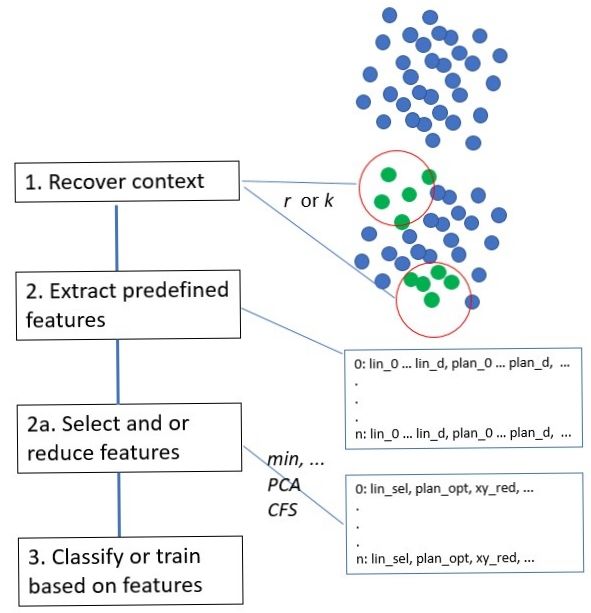
The International Archives of the Photogrammetry, Remote Sensing and Spatial Information Sciences, Volume XLIII-B2-2020, 2020
XXIV ISPRS Congress (2020 edition)
or principal component analysis (PCA). There are hybrid approaches e.g. (Landrieu, Boussaha, 2019),
(Landrieu, Simonovsky, 2018), which combine constant neigh-
The expectation is that the usage of the all-scale approach im- bourhood scale and optimised size of super-neighbourhoods called
proves the classification performance, due to its ability to integ- superpoints. Constant scale kNN neighbourhoods are used to
rate dynamically scaled context information. This improvement extract features for the unsupervised segmentation into super
comes on the cost of higher computational effort, which can be points. The number of points withing the superpoints is de-
reduced by GPU computation or dynamic estimation of scales pendent on the number of neighbouring points showing similar
in the feature extraction part of a deep learning framework. feature values.
Existing multiscale approaches vary in extraction and classific- For (ii) and (iii) we have to calculate properties for different
ation methods like deep learning (Qi et al., 2017) (Guo, Feng, scales, either to select an optimal one or to use multiple of
2018) or classical models (Weinmann et al., 2013). All these them. This causes computational costs. The all-scale approach
approaches experience drawback from the so-called Hughes phe- leads to even higher computational costs; nevertheless, it can
nomenon (Hughes, 1968), namely the decreasing classification be covered with modern hardware. This allows us to investig-
accuracy for growing feature space dimensionality. The ap- ate the performance gain through the all-scale approach. The
proach of optimizing the scale per instance, in this case per clas- runtime optimization will be done in the future.
sified point, does not have this problem but it tends to converge
towards small scales and ignores the nearby context informa-
tion. 3. METHODOLOGY
In this work, we propose a strategy to use a large number of
scales and overcome the Hughes phenomenon by means of fea- A point cloud is an unordered and unstructured set of points.
ture selection or aggregation. The main goal of this evaluation Each point p ∈ R3 consists of 3 parameters and refers to a
is not the maximization of the classification performance, but position in metric space. We search for a mapping which as-
the analysis of the all-scale contribution to the classification signs each point in the point cloud to a semantic class. Utilizing
performance. Therefore we use a minimalist framework with given labels to a certain set of points we train a machine learn-
few geometrical features and simple classifiers. ing model to map the points to the semantic classes. This basic
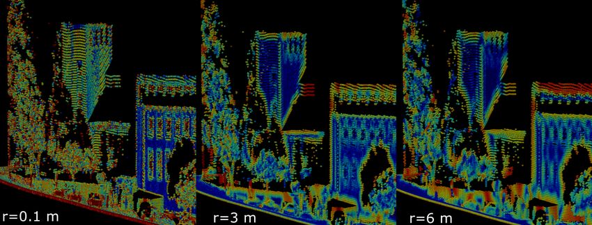
process consists of the following steps 1:
The remainder of this paper is structured as follows. In the next
Section 2 we will report the related work, in the Section 3 we
describe the full point cloud classification pipeline that we pro- 1. Recover context of a certain point by recovering its neigh-
posed in this research, in Section 4 we present the experimental bourhood with a single scale.
results, and making some conclusions of the study in Section 5.
2. Extract predefined features from the neighbourhood.
2. RELATED WORK 3. Classify or train a classifier based on the features.
The structure recovery from point clouds is based on neigh-
bourhood definitions using a certain scale parameter. There are We adopt this process by expending part 1 to recover a set of
three common strategies to handle the scale parameter (i) global neighbourhoods within a range of scales. We introduce after
single scale, (ii) global multiscale, (iii) one local scale per point. step 2 the feature selection and feature reduction as step 2a.
(i) This default strategy defines a single scale for the whole
dataset and depends on prior knowledge about the dataset. It
can be used with cylindrical (Filin, Pfeifer, 2005), spheric (Lee,
Schenk, 2002) (Linsen, Prautzsch, 2001) and kNN neighbour-
hoods. The scale is subject of meta-parameter optimisation and
have to be redetermined for each data set with differing prop-
erties. The static size of the scale makes it impossible to cover
relevant contexts for classes of different sizes, like for example
cars and buildings. This strategy has a limited generalisation
behaviour as the parameters have to be adapted to a certain data-
set.
(ii) Combination of several different global scales from (i) provides
implicitly information about changes between scales and al-
lows the framework to consider different scales (Niemeyer et
al., 2014) (Schmidt et al., 2014).
(iii) The scale of the neighbourhood selected for each point de-
pends on the properties of the neighbourhood. The scale can
be selected based on eigenentropy (de Blomley et al., 2016)
(Blomley et al., 2016). This strategy allows to generalise from
a specific data set, but still suffers from the disability to cap-
ture context from different scales, like for example a car has
tires (scale less than 1m) and appears almost always on the road Figure 1. Process overview
(scale of several meters).
This contribution has been peer-reviewed.
https://doi.org/10.5194/isprs-archives-XLIII-B2-2020-263-2020 | © Authors 2020. CC BY 4.0 License. 264The International Archives of the Photogrammetry, Remote Sensing and Spatial Information Sciences, Volume XLIII-B2-2020, 2020
XXIV ISPRS Congress (2020 edition)
3.1 Defining the Neighbourhood Eigenentropy:
In this paper, we consider two classical ways of defining the Eλ = −λ0 ln(λ0 ) − λ1 ln(λ1 ) − λ2 ln(λ2 ) (6)
neighbourhood of a point in a point cloud for feature extrac-
tion: first, a spheroid with a chosen radius, and second, neigh- has the valuation within the range [0, 1] where one indicates
bourhoods consisting of the k nearest neighbours in space. A maximal disorder in the neighborhood.
neighbourhood P is a subset of the point cloud and two dif-
ferent neighbourhoods can share (all) points depending on the R of k: Distance from query point to the furthest point in the
topology of the point cloud. The neighbourhood of pi ∈ R3 is neighbourhood. Considering a kNN neighbourhood this is the
referenced as Pi . distance to the k-th point. In the case of the ball-shaped neigh-
bourhood, it is the distance of the furthest point to the query
3.2 The Structure Tensor and Eigenvalue-Derived Features point. If there is no point in the radius this value is zero. In
order to be always able to calculate all features, we added an
As we are interested in describing the local geometry of the in cases when λ2 was zero.
neighbourhood of a point, the first step is to remove absolute
location information, by subtructing the centroid from the neigh-
bourhood. Otherwise the calculated eigenvalues would describe
the position of the neighbourhood. Then, we estimate the point
covariance matrix by organising a neighbourhood Pi in a n × 3
matrix A with n ∈ N number of points in PI . Finally, we
calculate λ0 , λ1 and λ2 from the eigenvalue decomposition of
AT A. This 3 × 3 matrix is called structure tensors for 3D point
clouds. The extracted three eigenvalues λ0 , λ1 , and λ2 are sor-
ted and normalised to fulfil λ0 >= λ1 >= λ2 >= 0 and
λ0 + λ1 + λ2 = 1 and derive the features listed below (Wein-
mann et al., 2013).
Eigenvalues:
λ0 , λ1 , λ2
The values of the eigenvalues correlate with the shape of the Figure 2. Eigenentropy as function of λ0 and λ1
neighboorhood, therefore we use them as three standalone fea-
tures. λ0 has a value in the range [1/3, 1]. λ1 is defined to be 3.3 Reference Classification System
smaller than λ1 and has the value in the range [0, 0.5]. Follow-
ing the definition is λ2 value in the range [0, 1/3]. With the feature extraction techniques from the previous sec-
tions, we can create a set of numeric features for each point
Linearity: based on a suitable definition of neighbourhood. The classifica-
λ0 − λ1 tion problem now consists of finding a machine learning model
Lλ = (1)
λ0 that can predict the class of a point given only these derived fea-
This feature has the valuation within the range [0, 1] where one tures. We perform a spatial split on the datasets to have train and
indicates maximal linearity. test sets, train various classifiers on the selected training data
and evaluate the performance of the trained classifier on the test
Planarity: set. In some cases, when hyper-parameter needs to be tuned, we
λ1 − λ2 apply another hold-out set, that is, we train on a training set, use
Pλ = (2)
λ0 a validation set to find the ideal hyperparameters and evaluate
the final performance on another spatially independent test set.
This feature has the valuation within the range [0, 1) where one
It is worth noting that a spatial split does not guarantee the inde-
indicates maximal planarity.
pendence of the distributions. According to Toblers law (Tobler,
Scattering: 1970), everything is related to everything, but near things are
λ2 more related than distant things. Translating to the situation of
Sλ = (3) spatial machine learning, this just means that it makes sense to
λ0
expect the dependencies between the spatially distant train and
This feature has the valuation within the range [0, 1] where one test sets to be smaller than if using just a random train test split
indicates maximal voluminous distribution. in which many of the points might be near to each other. Still,
the law tells us that the distributions are not independent, hence,
Omnivariance: actual performance values have to be consumed with care: they
Oλ = (λ0 · λ1 · λ2 )1/3 (4) are related to the same spatial dependency of the train and test
has the valuation within the range [0, 1] where one indicates sets. In many cases, the nature of the collection of the dataset
maximal omnivariance. implies that it comes from the same city similar architecture,
similar car manufacturers, similar street signage are examples
Anisotropy: of unavoidable correlations between the train and test sets.
λ0 − λ2
Aλ = (5) 3.4 Entropy-based Scale Selection
λ0
has the valuation within the range [0, 1] where one indicates The structure tensor of a neighbourhood describes the covari-
maximal Anisotropy. ance of this neighbourhood. This can be seen as a description
This contribution has been peer-reviewed.
https://doi.org/10.5194/isprs-archives-XLIII-B2-2020-263-2020 | © Authors 2020. CC BY 4.0 License. 265The International Archives of the Photogrammetry, Remote Sensing and Spatial Information Sciences, Volume XLIII-B2-2020, 2020
XXIV ISPRS Congress (2020 edition)
of a random process generating points. The predictability of R to determine which feature are useful. We define ρxc as the
these points can be captured by Shannons entropy by employ- average correlation between feature and class labels, ρxx as the
ing the Linearity, Planarity, and Scattering features from 3.2: average correlation between features and n as the number of
features. Then Relevance measure is defined as follows:
Edim = −Lλ ln(Lλ ) − Pλ ln(Pλ ) − Sλ ln(Sλ ) (7)
nρxc
R(X1...n , C) = p (8)
n + n(n − 1)ρxx
In fact, choosing k (the number of nearest points) such that this
information measure is minimized has been shown to work well
in practice (Weinmann et al., 2015). In addition, it is possible to 3.7 Feature Reduction
directly minimize the following expression avoiding the calcu-
lation of the features by using Eλ . Figure 2 illustrates the the- The problem of the correlated features described in the previ-
oretically possible distribution of the values. The eigenentropy ous section can as well be treated by means of principal com-
is minimal when λ0 is maximal and λ1 is minimal. Linearity is ponent analysis (PCA) (Hotelling, 1933). PCA reduces a h di-
the dominance of one dimension λ0 over the other two dimen- mensional space to an l dimensional space where h > l. The
sions. This dominance is described by planarity based on the reduction is based on the projection of the initial space to a
proportion of λ0 against λ1 and λ2 . As we aim to minimize the space defined by an orthonormal basis where the eigenvectors
eigenentropy we move toward cases where λ0 is large and the are defined by the direction of the largest variance of the data-
other two dimensions are small. In these cases, the normalized set. In our case we interpret each feature fi in feature set F ,
λ0 is describing approximately the linearity. Analogously λ1 with i < h ∩ N , as a dimension of the h-dimensional space. We
and λ2 approximate planarity and scattering. aim to reduce F to a lower l-dimensional space F 0 with h > l.
Let KF be the covariance matrix between all features of F . We
3.5 All-Scale Approaches calculate the eigenvalues of KF and select l eigenvectors with
largest eigenvalues. The dimensionality l is selected in a way
In this paper, we want to show that a scale-free approach is
that the reduced feature space F contains a certain fraction tv
feasible and provides comparable performance. There are two
of the variance of the original feature space F .
general approaches to remove the scale parameter from the sys-
tem. In any case, we are going to compute all features for a Random Forest (RF) is an ensemble classifier approach which
large set of scale parameters k or r. assumes that several weak classifiers compose into a better model
In our approach, all of those features provide a high-dimensional than a single strong classifier (Breiman, 2001). The weak clas-
classification problem with many highly-correlated features and sifiers can be trained based on bagging strategy (Breiman, 1996).
the classification system must take care to select suitable sub- A subset of the training dataset is selected randomly and a weak
sets of features. With respect to this problem, we propose to classifier is trained on this subset. The process is repeated a cer-
use Support Vector Machines with l1 and l2 regularization, as tain number of times, which generates an ensemble of different
they are known to deal well with high-dimensional classifica- weak classifiers. The aggregated hypothesis of this classifiers
tion problems, to perform a PCA on the set of features in or- provides a well-generalized prediction.
der to reduce the correlation between features, to use random Support Vector Machine (SVM) is a binary classifier which
forests and Correlation-based Feature Selection (CFS) (Hall, estimates a hyperplane to separate two classes in feature space
1999)to assess the feature importance in a first step and then linearly. Since not always two classes can be separated linearly
truncate the classification problem to include only the top fea- a kernel function can be introduced which maps training data
tures, and to empirically test the improved performance of the to a higher dimensional feature space. We use the radial basis
model trained on subset of features. function (RBF) as kernel. To apply SVM to multiclass prob-
A single aggregated feature for all values of k is determined by lems, the one against all approach (Chang, Lin, 2011) is used.
minimum, mean and maximum function. For each point and In this case, several classifiers are trained. Each learns how to
feature we determin the minimal values, for example we select separate one class from the others.
for each point from linearity values for all scales the minimal
value what results in a new feature min linearity . 4. EXPERIMENTAL SETUP
3.6 Feature Selection
4.1 Dataset
Our approach considers a large number of scales with a small
difference between the scales. This leads to highly correlated We test our framework on the Oakland dataset (Munoz et al.,
features for the kNN and even more for the ball-shaped neigh- 2009). It is a well-known dataset which was acquired by a
bourhoods. In case when we extend a kNN neighbourhood with mobile mappings system. The dataset contains scenes from an
a large k by only a few points the shape of the neighbourhood urban area. In our experiments, we used the classification with
changes only little and the resulting features are highly correl- 5 classes. Those are the following. Facade: In general it can
ated. For the ball-shaped neighbourhoods, the problem is even be interpreted as a building. Load bearing: Mostly this class
more crucial. When increasing the radius only in little steps refers to roads and sidewalks. Utility pole: This can be a tree
there is a high probability of not including additional points in trunk or artificial pole like a lamppost. Scatter misc: This class
the bigger neighbourhood and the calculated features remain consists of vegetation like tree crones, bushes or grass. De-
the same for a sequence of a sequence of scales. fault wire: This class refers to different wires in the scenes.The
data is subdivided authors in to three spatially disjoint subsets
In order to reduce the problems with correlated features, we use train, validate and test. The classes are highly imbalanced in
Correlation-based Feature Selection (CFS) (Hall, 1999), a mul- this dataset. Especially the classes facade and load bearing are
tivariant filter-based approach which uses Relevance measure over-represented.
This contribution has been peer-reviewed.
https://doi.org/10.5194/isprs-archives-XLIII-B2-2020-263-2020 | © Authors 2020. CC BY 4.0 License. 266The International Archives of the Photogrammetry, Remote Sensing and Spatial Information Sciences, Volume XLIII-B2-2020, 2020
XXIV ISPRS Congress (2020 edition)
4.4 Feature Selection:
In the next step, we extract the features from the optimal scale
neighbourhoods given by on the minimal entropy criteria de-
scribed earlier. The feature sets for the two neighbourhoods
definitions (opt r05) and (opt k) are extracted by selecting the
scale with minimal eigenentropy for each point. The ball-shaped
eigenentropy values are often zero for small scales of the ball.
Figure 3. Label distribution in trainings dataset
In sparse areas or for small scales the number of retrieved points
is too small. Therefore, we constrained the selected scale to a
4.2 Feature calculation : minimum radius of 0.5m. Overall this set contains 12 features
with per-instance varying neighbourhood scales.
We calculate the features for two definitions of the neighbour- We apply CFS to the training subsets of the union over all r,
hoods the kNN and the ball-shaped. For each point in the data- opt r, agr r and the union over all k, opt k, agr k. The result-
set, we determine the particular neighbourhood. The stated goal ing feature sets (cf s r) and (cf s k) contain each 59 features.
of this paper is to work with all the neighbourhoods. The prac-
tical interpretation of this goal is that we calculate the features 4.5 Measures
for neighbourhoods in certain range [start, end]. A step is a
size between two adjacent neighbourhoods. For each of the We evaluate the performance of the trained classifiers using
scales, we calculate all features described in section 3.2 For the measures precision, recall, f1 score, accuracy. We define
the KNN neighbourhoods, we use the parameters start = 8, T P, T N, F P, F N ∈ N as number of correctly classified points
end = 200 and step = 2 points. For the ball-shaped neigh- as a certain class, number of correctly not classified points as
bourhoods, we use the parameters start = 0.1, end = 8 and a certain class, number of points falsely classified as certain
step = 0.08 meter. The selected parameter values are based on class, and finally number of points falsely not classified as cer-
scale sizes from (Weinmann et al., 2013) and (Niemeyer et al., tain class.
2014). The run time for the calculation of the features for the
TP + TN
given parameters is 9 minutes for 36932 points and 35 minutes Accuracy = (9)
TP + TN + FP + FN
for 91515 points (CPU Intel I7-7700 and 16GB RAM).
Overall Accuracy (OA) is the ratio of the all correctly predicted
The feature calculation results in the following feature sets: points to the all points with prediction.
TP
P recision = (10)
1. All scales and all features of the ball-shaped neighbour- TP + FP
hood set (all r). Overall 1100 features per instance.
2. Four single scales and all features of the ball shape neigh- TP
Recall = (11)
bourhood set (r = x) x ∈ {0.1, 2, 4, 8}m. Overall 11 TP + FN
features per instance. 2 ∗ P recisionRecall
3. All scales and all features of the kNN neighbourhood set F1 = (12)
P recision + Recall
(all k). Overall 1100 hundred features per instance.
4. Four single scale and all features of the kNN neighbour-
hood set (k = x) x ∈ {10, 50, 100, 200} points. Overall 5. RESULTS AND EVALUATION
11 features per instance.
5.1 Feature Calculation:
Figure 4 shows the point cloud coloured by the linearity value
The four single scale sets for both neighbourhood are distrib-
of each point. Colourisation changes depending on the scale
uted evenly over the investigates scale ranges, what should us
which was used for the calculation of the feature. On the left
allow to show the effects of missing context and blurring on the
side we can see how a scale of radius 0.1 leads to high values on
classification performance.
the planar wall of the tower, because the scale captures single
scan lines. The two larger scales do not have this problem, but
4.3 Feature Reduction: in this configuration the linear structures of the windows are not
identified.
Based on all r and all k feature sets we generate simple ag-
Figure 5 shows three features as function of radius of the ball-
gregated feature set (agr r) and (agr k) by calculating min-
shaped neighbourhood. The features are averaged over all points
imum, mean and maximum of the feature value series over the
of the training dataset.
scale of the neighbourhoods. In addition, we use the neigh-
bourhood scale of the max, mean or min feature value as a new 5.2 Feature Selection:
aggregated feature.
When using the minimal entropy approach, the scale of the se-
The PCA reduced feature sets (pca r) and (pca k) are gener- lected neighbourhood tends to be minimized as well. As we
ated from the all r and all k feature sets. The reductions are can see at the diagram showing the distributions of the selected
determined by applying PCA with to the training set, result- scales this approach is able to select intermediate scales for the
ing in 30 combined features in (pca r) set and 16 features in kNN neighbourhoods and for the ball-shaped neighbourhoods
(pca k) set the tv = 0.95 (see 3.7). if use the 0.5m radius constrained.
This contribution has been peer-reviewed.
https://doi.org/10.5194/isprs-archives-XLIII-B2-2020-263-2020 | © Authors 2020. CC BY 4.0 License. 267The International Archives of the Photogrammetry, Remote Sensing and Spatial Information Sciences, Volume XLIII-B2-2020, 2020
XXIV ISPRS Congress (2020 edition)
Feature Ball Shaped r [m]
lambda1 –
lambda2 r= {0.42, 0.50, 0.58, 0.74, 1.23, 1.38,
1.46, 1.54, 2.34, 2.42, 2.50, 2.82,
4.18, 7.62}
planearity r= {0.42, 0.50, 0.58, 0.66, 0.74, 0.90, 0.98}
scattering r= {0.50, 0.58, 0.74, 0.90, 1.06}
anisotropy –
omnivariance r= {0.41, 0.73, 1.14, 1.22}
eigenentropy r= {0.49, 0.58, 0.73, 0.81, 0.89,
0.97, 1.05, 1.14, 1.53, 2.01}
Figure 4. Points coloured by linearity values in different scales: chg of curv r= {0.58, 1.38}
0.1, 2 and 3, from left to right; (Red: 1, Blue: 0) r of k –
optentropy {r of k}
min feature {lambda2 step, scattering step,
anisotropy, r of k}
max feature {lambda1, lambda2,
linearity step, planarity, scattering }
mean feature {lambda2, scattering, omnivariance,
anisotropy}
Table 2. CFS Selected Features - Ball Shaped
Figure 5. Linearity, Planarity and Eigenentropy as functions of
radius in meter. Horizontal axis shows the radius of the
neighbourhood in meters. Vertical axis shows the value of the
metrics.
Figure 6. Overall Accuracy - kNN neighbourhood
The features selected by CFS consist of simple eigenvalues like
lambdas as well as of the features from the agr r/k feature
set. Only a few features from the opt r/k feature set have been Figure 7 shows the overall results for all feature set configura-
selected. The selected features are similar for the kNN and ball- tion for the ball-shaped neighbourhoods. The results here vary
shaped neighbourhood. The selected scales are distributed over between 0.18 for RF and single scale of r = 8m and OA of
the considered interval. Furthermore, the aggregated features 0.89 generated by single scale feature set r = 2m and SVM.
based on entropy and min, max, mean features are included. The feature sets CF S and all have the OA of 0.89 and 0.88.
Feature kNN k [#]
lambda1 k= {64, 110, 184}
lambda2 k= {10, 14, 38, 40, 46, 58,
76, 194, 200}
planearity k= {16, 24, 26, 28, 58,
102, 122}
scattering k= {8, 10, 12, 14, 18, 122}
anisotropy k= {12, 18}
omnivariance –
eigenentropy k= {22, 24, 26, 30, 32, 38,
54, 60, 62, 114, 126}
r of k k= {14, 164, 180, 196, 200}
optentropy {min, lambda2,
scattering, r of k}
min feature {lambda1, lambda1 step,
scattering, anisotropy}
max feature {lambda2, planarity}
mean feature {planarity, scattering, omnivariance}
Figure 7. Overall Accuracy - Ball-shaped neighbourhood
Table 1. CFS Selected Features - kNN
5.3 Classification The unweighted F1 score overview for the kNN neighbour-
hoods is shown in figure 8. The results in this diagram have
Figure 6 shows the overall accuracy results for all feature set the same tendencies as the values in figure 6, but all values
configuration for the kNN neighbourhoods. The values are sim- are lower. Analogously behave the results in figure 9 which
ilar, and the worst performance of 0.72 had the set with a single presents an overview of unweighted average F1 scores for the
scale k=10. The feature sets CF S and all provided the best and ball-shaped neighbourhoods. The highest values generated RF
equal results of 0.86. models with feature sets CF S and all.
This contribution has been peer-reviewed.
https://doi.org/10.5194/isprs-archives-XLIII-B2-2020-263-2020 | © Authors 2020. CC BY 4.0 License. 268The International Archives of the Photogrammetry, Remote Sensing and Spatial Information Sciences, Volume XLIII-B2-2020, 2020
XXIV ISPRS Congress (2020 edition)
Figure 8. F1 - kNN neighbourhood
Figure 11. F1 - Ball-shaped neighbourhood, class wise
performance of the SVM
Precision Recall F-Measure
cfs r all r cfs r all r cfs r all r
facade 0.52 0.47 0.63 0.60 0.57 0.52
load bearing 0.97 0.97 0.94 0.93 0.95 0.95
utility pole 0.18 0.25 0.41 0.41 0.25 0.31
scatter misc 0.97 0.95 0.82 0.79 0.88 0.87
default wire 0.04 0.04 0.82 0.87 0.07 0.08
Weighted Avg. 0.93 0.92 0.89 0.88 0.90 0.90
Table 3. Performance measures of the best performing
configurations: Ball-shaped neighbourhoods, RF
5.4 Analysis and Evaluation of neighborhood structures
Figure 9. F1 - Ball-shaped neighbourhood
Overall results show similar performance as the results of (Wein-
mann et al., 2015). Direct comparison is not possible due to the
The figures 10 and 11 show the F1 scores per class for the ball- different feature sets, nevertheless we conclude correctness of
shaped neighbourhoods in combination with RF and SVM. The our introduced framework, from the similarity of the results.
class load bearing is predicted with most homogeneous results
and reaches several times values of more then 0.90. The class 5.4.1 Performance of Single Scale Neighbourhoods Ex-
scatter misc has similar results except the very poor perform- periments with single scale feature sets show typical behaviour
ance for the smallest single scale r = 0.1m. A high variation of low performance for small scales due to the lack of context
of results we can see for the class f acade with maximal F1 information for the classification. Large scales have decreasing,
score of 0.57 for CF S feature set combined with RF. The class or at least not improving performance as can be expected from
utility pole has a poor performance for the single scale con- the blurring effect (compare figures 6, 7, 8 and 9). The OA score
figuration and the best F1 score of 0.31 fore the all feature set. of the r = 2 feature set combined with SVM is high and even
The worst F1 scores, compared to other classes, both models the best in its series (with an accuracy of 0.89), nevertheless it
reached on predicting the class def ault wire. The best res- should not be overestimated. The unweighted F1 score, which
ult for this class is 0.13 and it was reached by SVM applied to is not biased by over represented classes like load bearing and
opt.Entr feature set. scatter misc, for the same configuration is out performed by
the CF S and all feature sets in combination with RF.
5.4.2 Performance of all Scale Neighbourhoods Overall
results show that the usage of scale range outperforms markedly
single scale feature sets and and the optimal entropy feature
set is outperformed by all configurations of the CF S and all
feature sets, achieving accuracies in the range of 0.86 to 0.90.
Exception of this trend is the result for prediction of the class
def ault wire. The property of the optimal entropy approach
to converg towards large λ0 and therefore linear feature allows
better prediction for the linear objects. The relevance of the sev-
eral scales is although shown by the features selected by CFS.
The scales this features are distributed over the whole range of
Figure 10. F1 - Ball-shaped neighbourhood, class wise the investigated scales (see 2).
performance of the Random Forest
6. CONCLUSION
Table 3 show the direct comparison between the two best per-
forming configuration CF S and all feature set which are both The best performance was achieved using the all r and cfs r
combined with the RF. Both feature set lead to similar result feature sets. The all r feature set consists of a large number of
except the bold entries. features in different scales and provides context as well as detail
This contribution has been peer-reviewed.
https://doi.org/10.5194/isprs-archives-XLIII-B2-2020-263-2020 | © Authors 2020. CC BY 4.0 License. 269The International Archives of the Photogrammetry, Remote Sensing and Spatial Information Sciences, Volume XLIII-B2-2020, 2020
XXIV ISPRS Congress (2020 edition)
information to a classifier. This information is capable of im- Hackel, T., Wegner, J. D., Schindler, K., 2016. Fast semantic
proving the classification performance, however on the costs of segmentation of 3D point clouds with strongly varying dens-
computation time. In cases when the optimal scale is selected ity. ISPRS annals of the photogrammetry, remote sensing and
based on the range of precomputed features of different scales, spatial information sciences, 3, 177–184.
it is reasonable to use not only one optimal scale but several. Ei-
genentropy along the scales tends to have several local minima Hall, M. A., 1999. Correlation-based feature selection for ma-
which could be used instead of selecting a single scale based chine learning.
on global minima. The feature selection with CFS leads to a
Hotelling, H., 1933. Analysis of a complex of statistical vari-
slight improvement of performance. The selected feature scales
ables into principal components. Journal of Educational Psy-
subsample the scale intervals with a resulting higher delta scale.
chology, 24(6), 417–441.
This empirical delta scale should be considered in future exper-
iments to reduce calculation time. Hughes, G., 1968. On the mean accuracy of statistical pattern
recognizers. IEEE Transactions on Information Theory, 14(1),
The all-scale approach improves classification performance. In 55–63.
order to be practicable, the calculation time must be enhanced
using GPU based computation and incremental calculation of Landrieu, L., Boussaha, M., 2019. Point cloud oversegmenta-
features along with the scale interval. State of the art for the tion with graph-structured deep metric learning. Proceedings of
semantic label of point clouds is provided by the deep learn- the IEEE Conference on Computer Vision and Pattern Recog-
ing networks, which although employ neighbourhood and scale nition, 7440–7449.
definition. Especially approaches like (Landrieu, Boussaha, 2019)
and (Landrieu, Simonovsky, 2018) using only one constant scale Landrieu, L., Simonovsky, M., 2018. Large-scale point cloud
size to calculate features indicating similarity of points, can be semantic segmentation with superpoint graphs. Proceedings of
extended with an all scale-feature extraction. Integration of the the IEEE Conference on Computer Vision and Pattern Recog-
all-scale approach should improve performance of such models. nition, 4558–4567.
Lee, I., Schenk, T., 2002. Perceptual organization of 3D sur-
face points. International Archives Of Photogrammetry Remote
ACKNOWLEDGEMENTS
Sensing And Spatial Information Sciences, 34(3/A), 193–198.
This work was partially funded by the Federal Ministry of Edu- Linsen, L., Prautzsch, H., 2001. Local versus global triangula-
cation and Research, Germany (Bundesministerium für Bildung tions. Proceedings of Eurographics, 1, 257–263.
und Forschung, Förderkennzeichen 01IS17076). We gratefully
acknowledge this support. Munoz, D., Bagnell, J. A., Vandapel, N., Hebert, M., 2009.
Contextual classification with functional max-margin markov
networks. 2009 IEEE Conference on Computer Vision and Pat-
REFERENCES tern Recognition, IEEE, 975–982.
Niemeyer, J., Rottensteiner, F., Soergel, U., 2014. Contextual
Blomley, R., Jutzi, B., Weinmann, M., 2016. Classification Of classification of lidar data and building object detection in urban
Airborne Laser Scanning Data Using Goemetric Multi-Scale areas. ISPRS journal of photogrammetry and remote sensing,
Features And Different Neighbourhood Types. ISPRS Annals 87, 152–165.
of Photogrammetry, Remote Sensing & Spatial Information Sci-
ences, 3(3). Qi, C. R., Yi, L., Su, H., Guibas, L. J., 2017. PointNet++: Deep
Hierarchical Feature Learning on Point Sets in a Metric Space.
Breiman, L., 1996. Bagging Predict-
ors. Machine Learning, 24(2), 123–140. Schmidt, A., Niemeyer, J., Rottensteiner, F., Soergel, U., 2014.
http://link.springer.com/10.1023/A:1018054314350. Contextual classification of full waveform lidar data in the Wad-
den Sea. IEEE Geoscience and Remote Sensing Letters, 11(9),
Breiman, L., 2001. Random forests. Machine learning, 45(1), 1614–1618.
5–32.
Tobler, W. R., 1970. A computer movie simulating urban
Chang, C.-C., Lin, C.-J., 2011. LIBSVM: A library for support growth in the Detroit region. Economic geography, 46(sup1),
vector machines. ACM transactions on intelligent systems and 234–240.
technology (TIST), 2(3), 1–27. Weinmann, M., Jutzi, B., Hinz, S., Mallet, C., 2015. Semantic
point cloud interpretation based on optimal neighborhoods, rel-
de Blomley, R., Jutzi, B., Weinmann, M., 2016. 3D semantic
evant features and efficient classifiers. ISPRS Journal of Photo-
labeling of ALS point clouds by exploiting multi-scale, multi-
grammetry and Remote Sensing, 105, 286–304.
type neighborhoods for feature extraction. GEOBIA 2016.
Weinmann, M., Jutzi, B., Mallet, C., 2013. Feature relevance
Filin, S., Pfeifer, N., 2005. Neighborhood systems for airborne assessment for the semantic interpretation of 3D point cloud
laser data. Photogrammetric Engineering & Remote Sensing, data. ISPRS Annals of the Photogrammetry, Remote Sensing
71(6), 743–755. and Spatial Information Sciences.
Guo, Z., Feng, C.-C., 2018. Using multi-scale and hierarch-
ical deep convolutional features for 3D semantic classification
of TLS point clouds. International Journal of Geographical In-
formation Science, 1–20.
This contribution has been peer-reviewed.
https://doi.org/10.5194/isprs-archives-XLIII-B2-2020-263-2020 | © Authors 2020. CC BY 4.0 License. 270You can also read