NEMO 4.0 performance: how to identify and reduce unnecessary communications - E. Maisonnave, S. Masson* - Cerfacs
←
→
Page content transcription
If your browser does not render page correctly, please read the page content below
NEMO 4.0 performance:
 how to identify and reduce
unnecessary communications
  E. Maisonnave, S. Masson*

* Sorbonne Universités -CNRS-IRD-MNHN,
    LOCEAN Laboratory, Paris, France

          TR/CMGC/19/19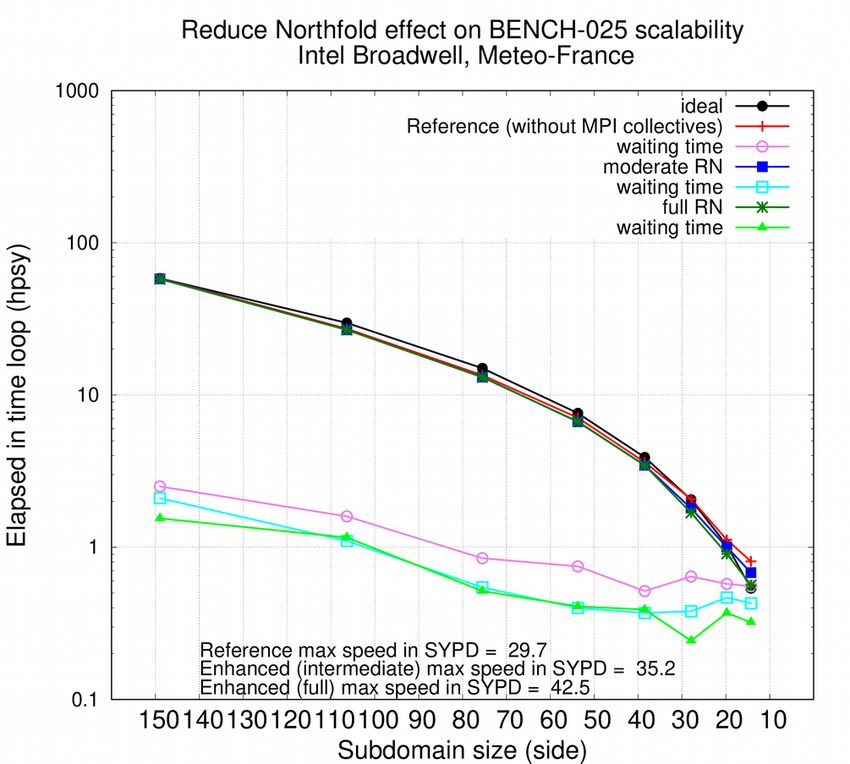
Abstract

A non-intrusive instrumentation of the NEMO code and the development of a simplified
configuration (called BENCH) brought information about MPI communications cost and
structure. It helped us to identify the most appropriate incremental developments that model
needs to enhance its scalability. We prioritised the reduction of extra calculations and
communications required at the North Polar folding, the grouping of boundary exchanges and
the replacement of global communications by alternative algorithms. Appreciable speed up (x2
in some cases) is measured. Scalability limit is pushed below a size of 7x7 grid points per sub-
domain, showing that the limitation of the North Polar folding solution can be compared with
the supposed icosahedral grid one. We consider that scalability is not the major well of future
performance gain, neither horizontal resolution increase, whereas potentiality of extra
developments accelerating cache access (horizontal domain tiling and single precision
computations) is favourably evaluated. Taking note of the limited technological gain between
the two 6-month old and 4-year-6-month old machines we operated, in order to avoid future
net decrease in computing performance, we recommend from now to limit new expensive code
developments to what technology and engineering are able to sustain.
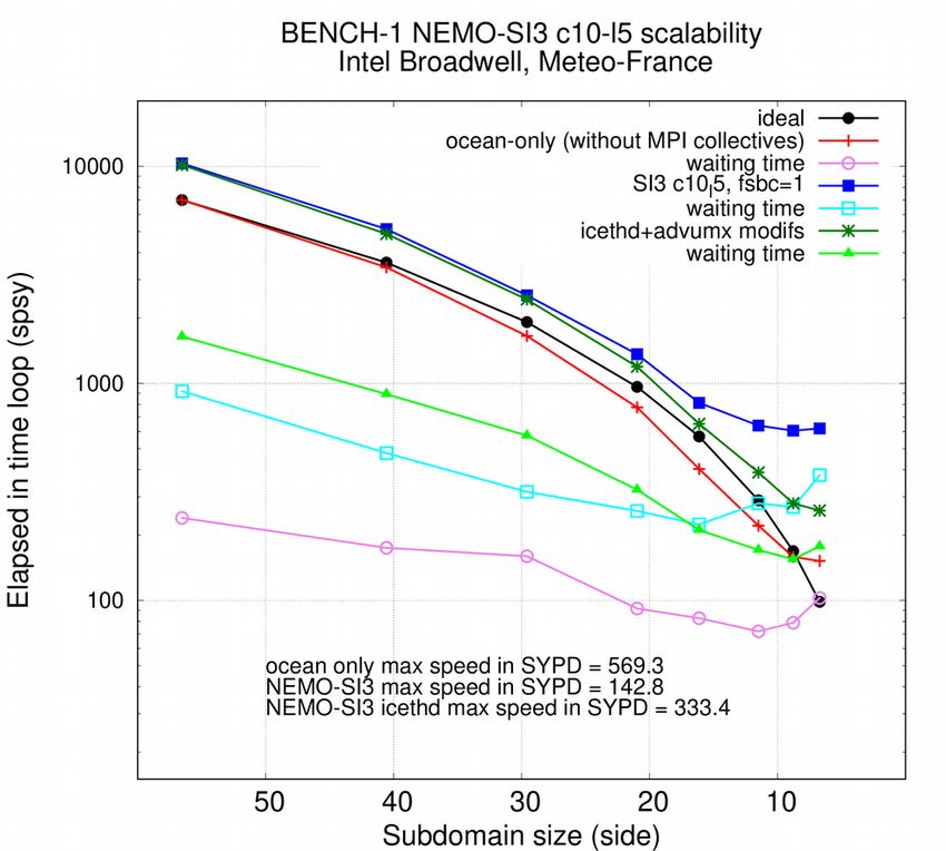
Table of Contents
1.Light code instrumentation dedicated to calculation / communication ratio measurement........4
2.BENCH: a simplified NEMO configuration for realistic performance analysis.....................................6
3.Experimental set-up............................................................................................................................................................. 7
    3.1.Methodology................................................................................................................................................................... 7
    3.2.BENCH performance analysis...............................................................................................................................7
4.Enhancement of North folding exchanges..............................................................................................................9
5.Other enhancements of OPA scalability..................................................................................................................11
6.Enhancement of SI3 scalability....................................................................................................................................... 12
7.Enhancement in TOP-PISCES model...........................................................................................................................14
8.Performance........................................................................................................................................................................... 14
9.Conclusion and perspectives.......................................................................................................................................... 16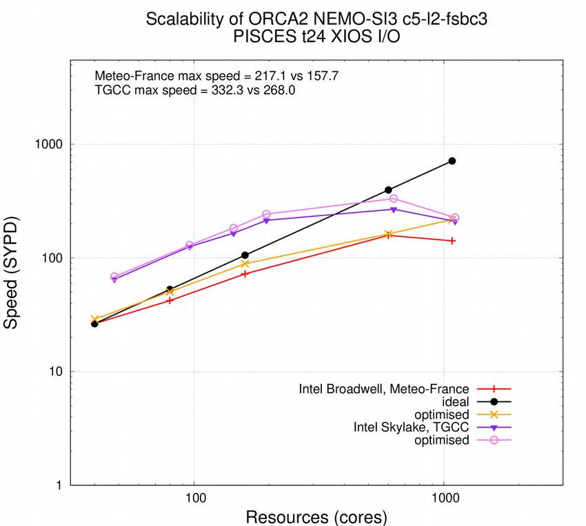
The cost of MPI communications is clearly identified as the most important factor of scalability
limitation of the NEMO model (e.g. Tintó Prims et al. 2018 [1]). Any new scalability improvement
in this model requires to carefully identify the place of the most costly MPI exchanges in the
code, to characterise their utility, before being able to propose a strategy of algorithm
modification, a communication reduction or a simple removal.

 1.       Light code instrumentation dedicated to calculation /
      communication ratio measurement

In NEMO, MPI communications are wrapped in a small number of high level routines co-located
in a single FORTRAN file (lib_mpp.F90). This code structure strongly facilitates a quick and
non intrusive instrumentation for a study dedicated to the MPI communication structure.
Basically, the NEMO communication library provides functionalities for horizontal halo
exchange and global averages or min/max operation between all horizontal subdomains. Every
halo exchange of any variable of the code necessarily needs to be done through the generic
“ROUTINE_LNK”. The global operations (sum, min/max) are also located in a few number of
routines, that can be also gathered following the same generic strategy (one routine fits all
argument kinds – integer/float/double, 2D/3D arrays - With very little code changes focused at
these positions, it is possible to identify and characterise, for further modification, the whole
MPI communication pattern. This instrumentation does not replace existing external solutions
like “extrae-paraver” described in Tintó Prims et al. 2018. The amount of information collected
by our solution is much smaller, and the possibilities of analysis reduced, but we are able to
deliver without any external library, without additional computing cost or additional post-
processing, a synthetic information for any kind of machine.

Because of some initial coding assumptions of the existing internal timing library routine
(timing.F90), we prefer not to modify and re-use its functionalities, but to slightly instrument
the ROUTINE_LNK generic interface with MPI_Wtime calls. Following the strategy already
deployed to estimate the coupled system load imbalance [2], a counter of the time spent in MPI
routines, also called “waiting time”, is incremented at any call of a MPI send or receive
operation in one hand, and at any MPI collective operations on the other hand. Symmetrically,
a second counter is filled outside these two kind of operation. Only two informations per core
are collected in two real scalar variables: the cumulated time spent to send/receive/gather or
(mostly) wait MPI messages and the complementary period of other operations (named
“calculations”).

The strategic position of our instrumentation allows to not only estimate the time spent in the
communication routines but also to identify their calling routines and the size and kind (2D/3D
or pointers of 3D arrays) of exchanged halo arrays. The calling of any lbc_lnk or MPI-
collective subroutine is modified to communicate, via sub-routine argument, the name of the
calling routine. A collection of these names is performed during the first time step of the
simulation. The second time step (which could be the second coupling time step when sea-ice
or bio-geo-chemistry model is enabled) produces the listing of the calling tree and the size of
the exchanges in a dedicated output file called communication_report.txt. We produce
below the content of such analysis for an ocean/sea-ice simulation: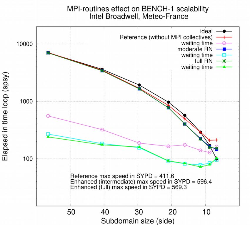
------------------------------------------------------------
  Communication pattern report (second oce+sbc time step):
  ------------------------------------------------------------

 Exchanged halos : 773
 3D Exchanged halos : 93
 Multi arrays exchanged halos : 163
   from which 3D : 22
 Array max size :      20250

  lbc_lnk called
 -    1 times by   subroutine     usrdef_sbc
 -    1 times by   subroutine     icedyn
 -    2 times by   subroutine     icedyn_rhg_evp
 -    1 times by   subroutine     icedyn_rdgrft
 -  483 times by   subroutine     icedyn_rhg_evp
 -   76 times by   subroutine     icedyn_adv_umx
 -    1 times by   subroutine     icethd
 -    1 times by   subroutine     icecor
 -    2 times by   subroutine     iceupdate
 -    2 times by   subroutine     zdfphy
 -    4 times by   subroutine     ldfslp
 -    1 times by   subroutine     divhor
 -    2 times by   subroutine     domvvl
 -    1 times by   subroutine     dynkeg
 -    1 times by   subroutine     dynvor
 -  177 times by   subroutine     dynspg_ts
 -    1 times by   subroutine     divhor
 -    2 times by   subroutine     domvvl
 -    1 times by   subroutine     traqsr
 -    1 times by   subroutine     trabbc
 -    6 times by   subroutine     traadv_fct
 -    2 times by   subroutine     tranxt
 -    1 times by   subroutine     dynnxt
 -    3 times by   subroutine     domvvl

 Global communications :    1
 -    1 times by subroutine icedyn_adv_umx

  -----------------------------------------------

During the second time step, it is possible to substitute the model operations ( step routine)
by the MPI exchanges of the realistic sequence of halo communications. This skeleton of realistic
exchanges is useful to avoid processing the whole simulation and help to save computational
resources during tests, as recently experienced by Zheng and Marguinaud, 2018 [3]. In our case,
the skeleton can be automatically set up for any NEMO configuration (resolution, namelist, CPP
keys) during the first time step and applied during the rest of the simulation. The sequence of
the communications can be modified or the communication block even switched off on
purpose to estimate the effect of such modification to the model performance.

At the simulation end, we also produce (if ln_timing option is activated in the namctl
namelist) a separated counting, per MPI process, of the total duration of (i) halo exchanges for
2D/3D and simple/multiple arrays, (ii) global communication to produce global sum/min/max,
(iii) all other MPI independent operations, called ‘computing time’ and (iv) the whole simulation,
excluding first and last time step. This analysis is output together with the existing information
related to timing in NEMO (timing.output file). We produce below the first lines of this
analysis for the same ocean ice simulation:
  Report on time spent on waiting MPI messages
     total timing measured between nit000+1 and nitend-1
     warning: includes restarts writing time if output before nitend ...

     Computing         time   :      7.674150                      on MPI rank   :     1
     Waiting lbc_lnk   time   :     10.760121   (58.4 %)           on MPI rank   :     1
     Waiting global    time   :      0.000163   ( 0.0 %)           on MPI rank   :     1
     Total             time   :     18.437015   (SYPD:   533.887 ) on MPI rank   :     1
     Computing         time   :      5.714904                      on MPI rank   :     2
     Waiting lbc_lnk   time   :     12.721502   (69.0 %)           on MPI rank   :     2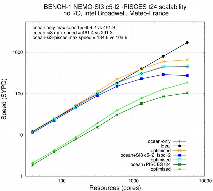
Waiting   global time :     0.000222 ( 0.0 %)           on MPI rank :             2
     Total            time :    18.439287 (SYPD:   533.821 ) on MPI rank :             2
(...)

 2.    BENCH: a simplified NEMO configuration for realistic
  performance analysis

The NEMO framework proposes various configurations based on the core ocean model OPA,
global (ORCA grid) or regional, with various horizontal and vertical resolutions. To this core
element, other modules can be added: sea-ice (.e.g. SI3) or bio-geo-chemistry (e.g. TOP-
PISCES). To deliver a synthetic message about the computing speed of the NEMO model, a
comprehensive performance analysis requires to investigate several resolutions / module sets.
On the other hand, such benchmarking exercise must be kept simple, since it is supposed to be
used by people with basic knowledge of model handling and physical oceanography.

This is why a new NEMO configuration was specifically developed for this study, and included in
the reference code with hope to simplify future benchmark activities related to computing
performance. This new configuration, called BENCH, is available in the tests/BENCH
directory of the last 4.0 code version. It is based on the existing GYRE configuration, with
modifications that make the measurements easier and increase its robustness.

GYRE horizontal grid is a simple cuboid, which dimensions can be easily changed by namelist
parameter. The lack of bathymetry ensures a relative numerical stability that allows various
numerical tests. All NEMO numerical schemes can be used. A selection of namelist parameters
is done to confer to GYRE the numerical properties that correspond to the chosen resolution.

GYRE does not include bathymetry (nor continents). However, in NEMO, calculations are
processed at each grid point (then mask is applied to take into account land grid point if any).
Consequently, the amount of calculations is the same with or without bathymetry and we
assume that this amount in GYRE (and BENCH) configurations is realistic. The only function
that our benchmark configuration cannot test is the removal of sub-domain entirely covered by
land points. We assume that the communication pattern would not be affected by this
characteristic.

The East-West periodical conditions and the North pole folding cannot be activated with
GYRE. These characteristics of the set of ORCA global grids (a consequence of the global
periodicity and of the bi-polar shape of the NEMO northern hemisphere representation) have
a big impact on performance and this is why the new BENCH configuration includes these
periodicity conditions, unlike GYRE. A simple change of the nn_perio namelist parameter
gives to the BENCH grid the ORCA periodic characteristics and reproduces the same
communication pattern between subdomains located on the Northern most part of the grid.

To be sure that these additional communications, compared to GYRE, are not affecting too
much the numerical stability of the model, we ensure in BENCH a bigger stability with constant
and small external forcing. External forcing is not read in files, which excludes evaluation of
input reading procedures from our performance analysis. The initial vertical gradient of the
density is minimised, but not removed, to let adjustment processes be launched and keep the
associated amount of calculations at a realistic value. In addition, the prognostic variables are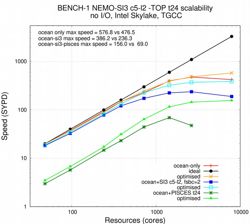
initialised with different values at each grid point, to ensure that reproducibility tests can be
effectively processed. Again, for stability reasons, these differences are minimised.

SI3 sea-ice or TOP bio-geo-chemistry can be activated in BENCH. An ORCA-like
representation of SI3 processes in the BENCH configuration implies a careful initial
temperature/salinity definition, in such a way that 1/5 of the domain would be covered, during
the whole simulation, with sea ice.

 3.          Experimental set-up

      3.1.    Methodology
A set of short simulations are produced with the Météo-France BULL supercomputer
“beaufix2”1. The total number of time step is adjusted to average enough information and
to minimise the exercise cost. Considering that initialisation and finalisation phases are excluded
of our measurement, the result dependency with respect to the time step number is supposed
to be small. At the opposite, it is important to minimise any disk access during the time loop. All
NETCDF Input/Output are disabled (no CPP key_iomput) and ASCII output are reduced to
the minimum.

To evaluate the benefit of our future modification, we will take measurement of a set of
simulations with various decompositions. Let’s emphasise here that performance is strongly
linked to the decomposition choice. This is why our BENCH implementation comes with a new
calculation of optimum decomposition values. We define the decomposition set which helped us
to determine scalability of our configurations, relying on the main assumptions that (i)
subdomain perimeter has to be minimised and (ii) the division rest of the total number of
subdomain by the number of core per node (CpN) has to be zero or close to CpN.

Part (i) of this algorithm was also implemented in the last official model release for all kind of
configurations, and enriched to take into account the land-only subdomains that are
automatically switched off.

      3.2.    BENCH performance analysis

Applying our measurement tool to the BENCH simplified configuration, a better picture of
scalability variations with resolution or machine is now available and it is even possible to clarify
their origin. On our current supercomputers, a normal usage of resources limits scalability
investigations to 1 or 0.25 degrees configurations. As shown in Figure 1-left, “waiting time” (MPI
communications + calculation load imbalance, pink line) is the limiting factor for BENCH-1 speed
(1 degree resolution, BENCH configuration, red line). The scalability limit is reached when the
length of the MPI subdomain sides falls below 10x10 grid points. In addition, the difference
between the fastest and the slowest calculations between MPI processes (orange line) gives an
idea of the total calculation spread, i.e. load imbalance, between subdomains. Its contribution to
the total waiting time is significant.

1     https://www.top500.org/system/178075
Figure 1, left: Scalability of BENCH-1 degree resolution configuration, considering total time to solution, in second
per simulated year, for several side length of MPI subdomains. Red line shows the total time to solution, pink line
shows the time spent to wait halo arrays (MPI messages), orange shows the difference between slowest and
fastest total calculations (excluding waiting time, see Figure 1, right) amongst MPI processes. Figure 1, right: total
time to solution but excluding time spent to wait halo arrays, for each MPI process, same unit, same model
configuration than left figure. The 6 measures are done with 6 different domain decompositions (domain side
length in legend)

Figure 2, left: Scalability of BENCH-1 configuration, considering total time to solution and time spent waiting MPI
messages (halos), same experiment than Figure 1-left (red and pink lines). In a second experiment, communications
are switched off. Total time to solution of this second experiment in shown in dark blue, with corresponding
calculations spread in light blue. Figure 3, right. In a third experiment, realistic communications are performed
every two time step only. Total time to solution of this second experiment in shown in dark green, with
corresponding waiting time in light green

Figure 1-right illustrates the imbalance of calculation time between the MPI processes. Processes
of the last two nodes shows extra calculations (arrays copies) of polar folding. They are the
origin of most of the total imbalance as plotted in Figure1-left (orange line). Additional analysis
(not shown) reveals that it is also at the origin of most of the extra waiting time (MPI
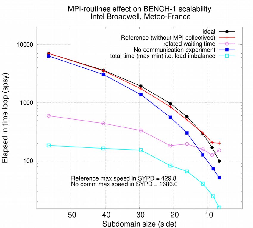
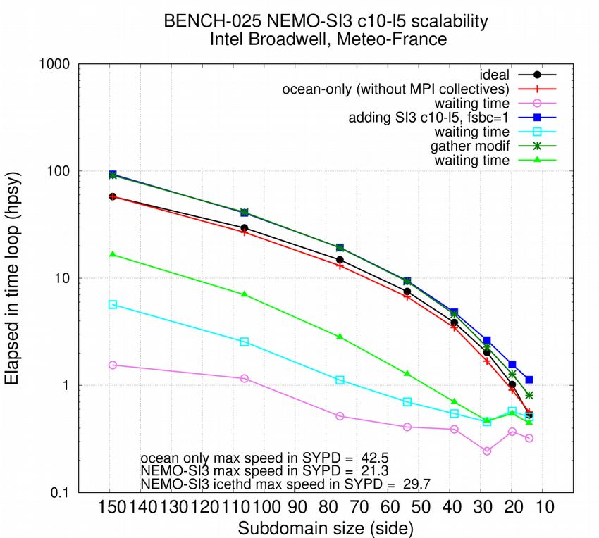
communication time). These analysis lead to prioritise our current model performance
enhancement work on polar folding effect reduction.

We also took benefit of the possibility to easily modulate the amount of communication to
sharply estimate the MPI exchange effect on scalability. Figures 2 compare time to solution and
calculation spread of our reference experiment with two others. In the first one, all halo
exchanges were switched off. In the second one, exchanges were performed every two time
steps only.

The first experiment quantifies the dominant effect of communication on performance at
every position of the scalability curve. As far as our measurement can be lead, the remaining
load imbalance cannot limit the scalability. The second experiment estimates the maximum
benefit of a possible implementation of a communication-reduced algorithm such as the so
called double halo (a two point wide halo is transmitted every two time step).

4.       Enhancement of North folding exchanges

The so-called North folding exchanges are made necessary by the particular tri-polar structure
of the ORCA global grids (see [4]). The uppermost subdomains located along the North pole
exchange their north-south halos between them. In this North folding area, the grid points of
the last line are duplicated (symmetry of type 5 or 6, currently used for ORCA1 discretisation).
With symmetry of type 3 or 4, used for ORCA025 or ORCA12 discretisation, the grid points of
the last but one line are symmetrically duplicated and the grid points of the last line are
duplicated on the last but two line. In addition, depending on the MPI decomposition, a
subdomain must have to be connected with two subdomains. These particularities, combined
with the C-Arakawa structure of variables, add extra arrays copies and extra communications
to the halo exchanges of the North fold area. Up to four lines, instead of one, are
communicated in the original NEMO code.

Simulation limited to realistic halo exchanges (skeleton) reveals that the size of exchanges data
has an impact on both calculation (mainly arrays copies) and MPI communications. A fine study
of North-South / East-West communication pattern reveals that only one or two lines
(depending on the grid type and the chose symmetry) are really necessary to update all grid
points in the North fold area. We call “moderate Reduced North folding (RN)” exchanges the
implementation that limits the exchanges to 1 to 2 lines. This implementation does not affect
the results.

A more aggressive reduction to one single communicated line is also implemented (“full RN”
exchanges). This can theoretically change the results because of the possible heterogeneity of
values that should be identical in restart variables on one hand, and the “triad” algorithm, used
e. g. in the total vorticity trend computation – energy and enstrophy conserving scheme - that
leads to reverse the operation order in the last 3 northernmost lines of the grid and introduce
a small difference in calculation results of two North-fold-symmetric subdomains, on the other
hand.

The two implementations are tested in the 4.0 version of the code (specific branch). The
experimental design is detailed at the previous chapter. The configuration is limited to the
ocean model only.

Effect on restitution time for each MPI process (subdomain) is plotted in Figure 3. We limit the
number of MPI ranks plotted to the very last 3 or 4 nodes, considering that North folding
effect only affects subdomains of the last 2 or 3 nodes. The reduction in elapsed time in sensible
at both BENCH-1 and BENCH-025 resolution. Resolution BENCH-12 is not shown due to the
lack of resources necessary to reach a sufficient communication time/calculation time ratio, but
the effect is supposed to be identical to the BENCH-025 one. From figures 4, we can deduce
that subdomain sizes of 5x9 (BENCH-1) and 17x24 (BENCH-025) are needed to estimate the
effect of our implementation.

Figure 3: Time to solution contributions per MPI process of computing (left) and waiting (right) routines, for
BENCH-1 (upper) -025 (lower). Last MPI ranks (from which North folding affected) are presented. Performance of
the initial implementation (red) is compared with the new algorithm of North fold halo exchange in moderate
(blue) and full (green) modes. Same configuration with no exchange at North fold (black) is also presented.

The computing time is reduced by our modification, in same proportion with both moderate
and full RN strategy: the additional time needed by North folding computations (mainly array
copies) cannot be estimated by comparison to a reference simulation led without any North
folding exchanges.

The reduction of MPI communication time is more difficult to estimate but can be roughly
deduced from waiting time measurements. At BENCH-1 resolution, it is hard to evaluate the
extra effect of full RN. At the opposite, a further reduction of waiting time is observed at
BENCH-025 resolution. This probably explains the extra speed up observed on Figure 4 (right)
from 35.2 SYPD (moderate RN) to 42.5 SYPD (full RN). We suppose that the reduction of MPI
messages size is more efficient with 17x24 subdomain size (BENCH-025) than with 7x9
(BENCH-1).

In both cases, a non negligible speed up (x 1.4) is obtained thanks to our strategy. The effect is
sensible at every decomposition but brings the better gains at scalability limit. Due to non
reproducibility of results in particular configuration (AGRIF), the moderate RN is eventually
included in the official release.

We deduce from Figure 3 that the North fold effect is no more the bottleneck that limits the
model scalability. At considered horizontal resolutions, the tri-polar grid does not introduce
more substantial extra load imbalance and could be compared to icosahedral grids.

Figure 4: Scalability of BENCH-1 (left) and BENCH-025 (right) configurations, considering total time to solution and
time spent waiting MPI messages (halos). Performance of the initial implementation (red/orange) is compared with
the new algorithm of North fold halo exchange in moderate (blue/cyan) and full (green/lime) modes. Same
configuration with no exchange at North fold (black) is also presented

5.         Other enhancements of OPA scalability

Other modifications are applied following two strategies: to group halo exchanges and to
remove unnecessary global communication.

During vorticity (dynvar.F90) calculation, halo communication are performed together for
all vertical levels (3D fields communication). Similarly, during tracer advection
(traadv_fct.F90), the 3 spatial components are grouped during communication.
Regarding global communications, a new procedure is implemented to check, at every time
step, that model prognostic quantities are bounded to realistic values. In this procedure, a local
(instead of global) check is performed and the decision to stop the simulation, after a local
output of the standard output.abort.nc file, is only taken by the MPI process affected by
the failure diagnostic. After the output of pre-abort prognostic variables, this single process
ends the simulation, stopping all MPI processes of the MPI_COMM_WORLD communicator. This
simultaneously ensures (i) a clean simulation stop, even in coupled mode, (ii) the output of local
quantities relevant to identify the crash origin (local output.abort.nc file) and (iii) the
removal of a global communication performed at each time step.

In addition, the number of unnecessary writing in disk is reduced:
    • The ln_ctl logical (unused in production mode) must be true to output the
        run.stat files
    • The time.step file is now written only by the first subdomain

6.         Enhancement of SI3 scalability

An analysis of the location and call frequency of halo exchanges and global communications in
the code (see figure 5, outer donut) reveals the major contribution of three routines of the sea
ice module (advection, rheology and thermodynamics). Only a change of the rheology
numerical scheme (iterative procedure needed to solve the momentum equation) could limit
the halo exchange frequency. Further analysis are necessary to this change. Modification of the
two other parts of the code are presented below.

                                         119478
                                                   74

                                          194761                                       icedyn_rhg_evp
                                                             177                       icedyn_adv_umx
                                                    177                                dynspg_ts
                485                                                                    dynvor
                                                                                       traadv_fct
                                                                                       domvvl
                                                                                       ldfslp
                          485                           77                             others
                                                                                       stpctl (global)
                                                                                       icedyn_adv_umx (global)

                                                    369

Figure 5: Occurrence of MPI-communication calls in an ocean/sea-ice configuration before (outer donut) and after
                                         (inner donut) optimisation

Advection trend calculation (TVD, ice_dyn_adv_umx routine), which includes 2D halo
exchange, is called for every layer (and every category). The reduction of communication
volume is here quite straightforward. We modify the adv_umx subroutine call: a single call is processed for all layers/categories and 3D (instead of 2D) arrays are exchanged during halo update. In ice thermodynamics, the computing of time evolution of snow and sea-ice temperature profiles (ice_thd_zdf_BL99 routine) needed a separate MPI communicator, dedicated to communications only between processor cover by sea-ice. Creation/removal of the communicator was performed at each time step and for each ice category. A global maximum, to evaluate the maximum value of a converging quantity, was the single function of the communicator. This global information ensured a number of convergence iterations that was independent of the MPI decomposition. We can keep this independence by calculating the convergence criterion and stop the convergence calculation for each grid point, independently of the others. This avoids the final global communication. The remaining global communications necessary to check, in sea-ice advection scheme, whether time splitting is necessary or not to avoid instability, are delayed by one time step, in order to perform one time step computations in the meantime. This strategy implies the coding of the checkpoint/restart procedure to preserve the “restartability” of the model. Finally, the extra cost of these “delayed communications” is practically reduced to zero. As show in Figure 5 (inner donut), all global communications and 1/3 of the halo exchanges are removed from ocean and ice code. As seen in Figure 6, this clearly push away the scalability limit. For clearer results, 10 categories and 5 layers are set in SI3 (instead of the usual 5 and 2 values), which is called at every ocean time step (instead of every 3 time step usually). The overall NEMO benefit depends on the SI3/OPA relative weight, which depends on the number of SI3 categories/layers, but the performance enhancement of the single SI3 model is mainly independent of these parameters. Figure 6: Scalability of BENCH-1 (left) and BENCH-025 (right) configurations, considering total time to solution and time spent waiting MPI messages (halos). Performance of the ocean only configuration (red/pink) is compared with the ocean-SI3 configuration, with initial (blue/cyan) and enhanced implementation (green/lime)
7.           Enhancement in TOP-PISCES model

Relying on the tools described above, the comprehensive study of global and boundary
communications in the TOP tracer module and biogeochemistry model PISCES reveals the
intensive use of global communications in 4 routines (see figure 7, outer donut).

                                      11 2

                                                      24

                                                                             trcrad
                         1                        1                          (outer:global/inner:loca
                                                                             l)
                                                                             trcstp (global)
                                                                             trcsbc
                                                            25               p4zsink (global)
                                                                             trcnxt
               96                                                            p4zflx (global)

                                     1

    Figure 7: Occurrence of MPI-communication calls in TOP/PISCES modules before (outer donut) and after (inner
                                              donut) optimisation

A removal of small negative quantities (numerical errors produced during tracer advection) is
performed in the trcrad routine. A global mean is necessary to compensate at every grid
point the quantities created by the negative values removal. A new system of compensation is
implemented: assuming that the negative values are always small, they can be spread on a 3x3
grid point local stencil, that can always be found (possibly on halo grid points) close to the
faulty values. This strategy leads to the removal of a global communication (but needs an
additional boundary exchange).

Following the same strategy than for ice and ocean, global checks performed in trcstp are
disabled in standard mode, and preserved only when the ln_ctl logical is set. Similarly,
global means, only needed for diagnostics, are called under IF statements: this removes the
communication call in pk4zflx routine. The p4zsink routine was entirely rewritten by
PISCES developers, that removes the last two global communications of the module. Finally, the
remaining halo communications in trcsbc can be grouped and reduced to one.

8.           Performance
We evaluate the benefit induced by the whole set of modifications between version 3.6 stable,
revision 10164 and version 4 of the code. Two set of scalability measurements are performed on
beaufix2 Météo-France and irene2 TGCC supercomputers, using the BENCH configuration
(resolution 1 and 0.25 degrees). This output-less configuration allows to isolate performance of
2    https://www.top500.org/system/179411
calculation and communications, without any interference of disk accesses. In parallel,
performance of the widely used ORCA2_ICE_PISCES configuration is also evaluated to see how
the impact of XIOS writing and disk accesses affect the results.
Figure 8: Scalability of BENCH-1 configuration, before and after optimisation described in this document, ocean
stand alone (red and orange), including sea-ice model with 5 categories and 2 layers, called every 2 ocean time
steps (dark and light blue) or including TOP-PISCES biogeochemistry, 24 tracers, called every time step (dark and
light green), on Météo-France (left) and CEA-TGCC (right) supercomputers.
In any cases, even though our processes are not sharing resources with other users jobs on our
exclusive computing nodes, results are largely dependant of the per-user bandwidth availability,
i.e. the machine load. Measurement error margin can be greater than 100% at extreme
scalability (>10,000 cores), when MPI communication time is a big contributor to the total
restitution time. Scalability plots presented in Figure 8 and 9 are established with the fastest
runs we could measure during the period of machine biggest availability (Christmas holidays).
This strongly mitigates the enhancements we got in any case (between x 1.15 to more than x 2
faster) but proves the ability of NEMO “polar-folding” communication scheme to lead 1 degree
ocean-only global simulations closer to the 1,000 SYPD target and to use ¼ degree ocean-only
global model under near perfect scalability conditions on the present day machines.
Comparison between 1 and 0.25 degrees configurations shows that scalability limit is only
reached at low resolution. From that, we deduce that only low resolution tests help us to
investigate the scalability limit of the model. The only extra information that BENCH-025
carries is that our present supercomputers can only process BENCH-025, BENCH-12 and
BENCH-beyond calculations below the scalability limit and other strategy of time to solution
reduction must be found elsewhere. Another consequence of this result is that the increase of
resolution is not a solution for a better use of the supercomputer resources: at 10,000 cores
limit, scalability will be nearly perfect for any global configuration above 0.25 degrees. At the
opposite, at 10,000 cores limit, the BENCH-12 subdomains, larger than the BENCH-025 ones,
will saturate the node memory caches and downgrade the performance.Figure 9: Same than 8, with BENCH-025 configuration
An uncertainty on measurement of the same kind than with BENCH (reinforced by disk
accessibility constraints) is observed with the full I/O low resolution configuration of the model
(see Fig 10). However, our communication reduction work is still sensible in this case.
Figure 10: Scalability of ORCA2_ICE_PISCES configuration, before and after optimisation described in this
document, sea-ice model with 5 categories and 2 layers, called every 3 ocean time steps (dark and light blue) and
TOP-PISCES biogeochemistry, 24 tracers, called every time step (dark and light green), including standard XIOS
output, on Météo-France (red and orange) and CEA-TGCC (violet and pink) supercomputers.
9. Conclusion and perspectives
The modifications we made lead to comfortable gains only if the model is used under very
special conditions: perfect condition of bandwidth use (nearly empty machine), no disk accesses,
model resolution fitted to reach scalability limit in present day supercomputers. At lowresolution, maximum speed is reached when the maximum per user number of resources are
requested. Considering that large requests are always delayed for longer periods than smaller
jobs, the actual performance (measured in ASYPD) of our enhanced model is probably less
alluring. As expressed in [5], a larger set of production runs would be necessary to better
estimate this difference. But it is clear that our enhancements are sensible mainly when
production conditions are unfavourable. At higher resolution, the scalability limit cannot be
reached, which strongly limit the impact of our modifications. To summarise, our enhancements
guarantees that the scalability limits of the tri-polar grided NEMO model can theoretically be
compared to other models/grids but, in practice, they lead to a modest 20 to 30% gain in
production conditions. This is why we consider that further optimisation should not focus on
scalability limits but investigate the enhancement conditions well below this limit.
Figure 11: Restitution (elapsed) time needed by the BENCH model to perform calculations per grid point (arbitrary
unit), for various sizes (square side) of the horizontal subdomain (including halo), allocated on each core of the
4x5/6x8 core node of beaufix2/irene supercomputers, in ocean-only, 75 vertical levels (upper-left plot),
ocean+SI3 ice module called every 2 time steps (upper-right plot), ocean+bio-geo-chemistry module including 24
tracers (lower-left plot) and all configurations together (lower-right plot)
In particular, a comparison of models (particularly ocean only) scalability with ideal scaling in
Figures 8 and 9 shows a super-scalability in the first part (below 500 to 1000 cores) of the plot.
A complementary analysis is produced to better identify its origin. In one node of our twomachines, we vary the size of each square subdomain attributed to each of the node cores (40 on beaufix2, 48 on irene) and we calculate the time spent to process calculations only (communications are switched off) for a fixed number of grid points. Results from Figure 11 prove that it is easier for a node, whatever NEMO configuration is (ocean only, ocean+ice or ocean+bio-geo-chemistry), to perform calculations with 10x10 than 100x100 horizontal subdomains. This probably reveals the sensibility of the model to the cache effect of the machine node. From this, we can infer that a judicious tiling of NEMO computations (the splitting of the sub-domain in smaller subdomain and execution within a loop, instrumented or not to add further OpenMP/OpenACC parallelism) could bring nearly a new factor two to the performance at low resource positions of the scalability plot at low global resolution (ORCA1) and any position for high resolutions. This work is complementary to and cumulative with the precision reduction already explored by [6]. We can also notice from our results that the maximum gain our implementation brings is comparable, or even larger, to the gain delivered by the machine upgrade (irene was made available 4 years after beaufix2), which shows the necessity of such algorithm adjustments to compensate the contemporary Moor’s law slowing down. It also makes clearer that such gain is now obtained with much less facility than one decade ago and, considering that sources of additional gain in the code are fewer and fewer, supercomputing should no more be considered as a cornucopia and strategies to limit new costly development in the code planned. Acknowledgements The authors strongly acknowledge the NEMO system and R&D teams, including Gurvan Madec, Clément Rousset, Olivier Aumont, Claire Lévy, Martin Vancoppenolle, Nicolas Martin and Christian Ethé, ATOS staff Louis Douriez, David Guibert and Erwan Raffin for their help and advices, and Michel Pottier and the TGCC hotline for their support on Météo-France and CEA-TGCC supercomputers. This work is part of the ESiWACE project which received funding from the European Union’s Horizon 2020 research and innovation program under grant agreement n° 675191. References [1] Tintó Prims, O., Castrillo, M., Acosta, M., Mula-Valls, O., Sanchez Lorente, A., Serradell, K., Cortés, A., Doblas- Reyes, F., 2018: Finding, analysing and solving MPI communication bottlenecks in Earth System models, J. of Comp. Science, https://doi.org/10.1016/j.jocs.2018.04.015 [2] Maisonnave, E., Caubel, A., 2014: LUCIA, load balancing tool for OASIS coupled systems,Technical Report, TR/CMGC/14/63, SUC au CERFACS, URA CERFACS/CNRS No1875, France [3] Zheng, Y. and Marguinaud, P., 2018: Simulation of the performance and scalability of message passing interface (MPI) communications of atmospheric models running on exascale supercomputers, Geosci. Model Dev., 11, 3409- 3426, https://doi.org/10.5194/gmd-11-3409-2018 [4] Madec, G., 2008: Nemo ocean engine. Note du pôle de modélisation, Institut Pierre-Simon Laplace (IPSL), France, no 27, ISSN no 1288-1619, § “Model domain boundary condition” [5] Balaji, V., Maisonnave, E., Zadeh, N., Lawrence, B. N., Biercamp, J., Fladrich, U., Aloisio, G., Benson, R., Caubel, A., Durachta, J., Foujols, M.-A., Lister, G., Mocavero, S., Underwood, S., and Wright, G., 2017: CPMIP: measurements of real computational performance of Earth system models in CMIP6, Geosci. Model Dev., 10, 19–34, https://doi.org/10.5194/gmd-10-19-2017 [6] Tintó Prims, O. and Castrillo, M., 2017: Exploring the use of mixed precision in NEMO. In Book of abstracts (pp. 52-54), Barcelona Supercomputing Center
You can also read