Irrigation of Young Cork Oaks under Field Conditions-Testing the Best Water Volume - MDPI
←
→
Page content transcription
If your browser does not render page correctly, please read the page content below
Article
Irrigation of Young Cork Oaks under Field
Conditions—Testing the Best Water Volume
Constança Camilo-Alves 1, * , Cati Dinis 1 , Margarida Vaz 2 , João M. Barroso 1 and
Nuno Almeida Ribeiro 1
 1    MED—Mediterranean Institute for Agriculture, Environment and Development & Departamento de
      Fitotecnia, Escola de Ciências e Tecnologia, Universidade de Évora, Pólo da Mitra, Ap. 94,
      7006-554 Évora, Portugal; cd@uevora.pt (C.D.); jmmb@uevora.pt (J.M.B.); nmcar@uevora.pt (N.A.R.)
 2    MED—Mediterranean Institute for Agriculture, Environment and Development & Departamento de
      Biologia, Escola de Ciências e Tecnologia, Universidade de Évora, Pólo da Mitra, Ap. 94,
      7006-554 Évora, Portugal; mvaz@uevora.pt
 *    Correspondence: calves@uevora.pt; Tel.: +351-266-760-822

 Received: 30 October 2019; Accepted: 7 January 2020; Published: 10 January 2020

 Abstract: This study is the beginning of the first long-term study on cork oak irrigation under
 field conditions, with a structural-functional approach. Cork oaks are currently facing disturbances
 affecting cork quality and quantity, jeopardizing the future of the economic sector. There is a need for
 new production techniques that maximize cork oak growth and vitality. In this study, irrigation was
 implemented in a new intensive cork oak plantations to test the best irrigation volume. The long-term
 goal is to improve tree growth with minimum water requirements. A 6 ha intensive plantation was
 installed in Coruche, Portugal. The experimental plot consisted of a subsurface drip fertigation
 system, buried 40 cm deep; with five independent irrigation treatments. It was tested four irrigation
 volumes during the dry period—21 weeks in the summer of 2016—ranging from 1.88 mm to 5.62 mm
 a week. Information on meteorological conditions, soil moisture profile and leaf stomatal conductance
 were gathered periodically and dendrometric measurements were performed before and after the
 treatments. Cork oaks’ structural and functional parameters were associated with irrigation volume
 Response to irrigation showed an inflection point in treatment 2, corresponding to a water supply
 of 3.12 mm per week: below the inflection point, stomatal conductance was reduced by 15% and
 relative diameter growth at the base was reduced by 10%. Stomatal conductance also showed a
 positive relationship with soil moisture below the irrigation tubes and with plants’ stem diameter.
 In conclusion, irrigation supply during the period of water stress improved function and structure
 of cork oaks seedlings under field conditions. These results suggest that irrigation can be a viable
 alternative to improve cork oak growth in afforestation and reforestation.

 Keywords: Quercus suber; tree growth; stomatal conductance; water relations; Mediterranean trees;
 precision irrigation

1. Introduction
     Cork oak (Quercus suber L.) is a sclerophyllous evergreen Mediterranean tree of high conservation
and socioeconomic value in its natural range area. This species covers about 2.2 M ha in the western
part of the Mediterranean basin, growing well in acidic soils on granite, schist, or sandy substrates [1].
The main product obtained from this tree is its outer layer, cork. Portugal produces about half of the
cork on the market (≈100,000 ton per year) and the remainder is mainly obtained in Spain, Morocco,
Argelia, Tunisia, Italy and France [2]. Cork oak forests and the derived silvopastoral systems are
ecologically and economically sustainable, serving as an important tool in preventing desertification [2].

Forests 2020, 11, 88; doi:10.3390/f11010088                                        www.mdpi.com/journal/forests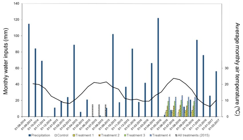
Forests 2020, 11, 88                                                                                 2 of 15

However, severe cork oak mortality events have repeatedly occurred in the Mediterranean basin since
the 1980s, disrupting the system in all its aspects [3–7]. Nowadays, cork oak dieback is considered a
complex multifactorial phenomenon involving the combination of several factors acting together [8],
where drought plays a role in causing trees to decline [3,4,9–11]. With a reduction in the raw material
the future of the cork industry may be jeopardized, principally the production of natural cork stoppers.
This is particularly relevant given that cork stoppers account for 70% of cork’s market value [2],
though they represent only 40% of cork production. In the search for new cork oak afforestation
techniques, private companies and institutional research centers have established several cooperation
projects between them. The long term goal is to develop sustainable production techniques capable of
reducing seedling mortality, increasing tree growth and favoring tree health. Empirical observations
and one cork oak field study [12] suggested that fertigation treatments may improve plant survival,
health, and growth in the early stages of development. Enhancing plant growth is a key factor for
research purposes due to the long period from planting until economically viable cork production.
By Portuguese law the circumference at breast height (CBH) of cork trees must reach 70 cm before
the first cork stripping, which usually occurs after 20 years’ age or more. Afterward, the cork can
be removed every 9 or 10 years. Under exceptional conditions, that period can be reduced to 7 or
8 years (Law 169/2001). Given that only the 3rd and subsequent harvests produce quality cork, a tree
only becomes economically viable after 40 years’ age or more. Therefore, the intent of this long-term
project is to reduce the time until the 1st or 2nd cork extraction through fertigation. Research must
also consider potential water supply constraints, particularly under current climate change scenarios.
Consequently, the major scientific question of the long-term project is: what is the lowest requirement
in water and fertilizers still improving cork oak growth? The objective is to maximize cork oaks’ growth
with efficient use of water, i.e., with as little water as possible. The hypothesis is that cork oaks have a
threshold in water requirements –both in time and “space” (quantity)—above which there will be no
significant growth. The specific aim of this study was to find the best irrigation volume for young cork
oaks in intensive plantations under a particular soil type. As the crop coefficient (Kc, a widely used
parameter for irrigation scheduling) of cork oaks is not known, the approach was the use of differential
irrigation treatments and monitoring water relations between soil-plant-air. Stomatal conductance is
considered to be related to plant water status in cork oak species [13–16] and can be used as a functional
trait parameter. With dendrometric measurements accounting for structural parameters, the expected
output will be a functional-structural response of the plants to different irrigation treatments.

2. Materials and Methods

2.1. Study Site
     The study took place at “Herdade do Corunheiro”, near Coruche, Portugal. The region is
characterized by a typical Mediterranean subhumid climate with hot and dry summers. The normal
annual average for rainfall in the region is 704 mm and for the annual temperature it is 15.1 ◦ C
(1971–2000, according to Portuguese Institute for Sea and Atmosphere data). Cork oaks cover 69% of
the forest area in this region, representing to the largest area occupied by this species in Portugal [17].
The farm is mainly covered with forest, especially by cork oaks. The 6-hectare experimental plot was
installed in 2014 in a former cropland for domestic use. A stream stands 130 m from the lower part of
the experimental area, with a difference in level of 6 m. The plot has a slope of about 7% facing 12◦
north. Soil profile evaluation and sampling were carried out in eight locations by a soil science expert
from the University of Evora: soil profiles were unstructured and presented sandy texture with loose
tenacity and friability, non-stickiness, no plasticity and minimal compaction. Samples were sent to a
specialized laboratory (the Agricultural Chemical Laboratory of the University of Evora) for physical
and chemical evaluation. More than 75% of the particles were gross sand (Table 1a). Organic matter
was very low (0.32%) and nitrogen was not detectable (Table 1b).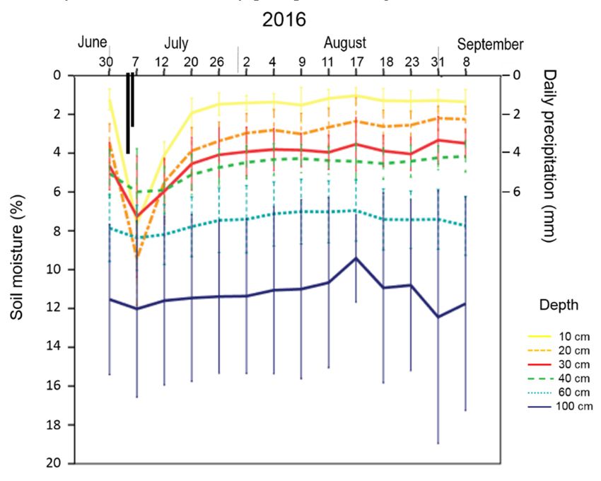
Forests 2020, 11, 88 3 of 15
Forests 2020, 11, x FOR PEER REVIEW 3 of 15
Table 1. Main results (Mean ± SD) of the physical (a) and chemical (b) properties of the soil profile at
eight experimental field locations.
Table 1. Main results (Mean ± SD) of the physical (a) and chemical (b) properties of the soil profile at
eight experimental field locations. a: Physical Properties
Density (g cm−3 ) Gross Sand (%) Fine Sand (%) Silt (%) Clay (%)
a: Physical Properties
1.60 ± 0.11 77.55 ± 3.48 11.47 ± 1.78 4.48 ± 0.97 6.50 ± 0.97
Density (g cm−3) Gross Sand (%) Fine Sand (%) Silt (%) Clay (%)
1.60 ± 0.11 77.55 ± 3.48 b: Chemical Properties
11.47 ± 1.78 4.48 ± 0.97 6.50 ± 0.97
O.M. (%) pH (H2 O) P2 O5 (ppm) N (%) K2 O b: Chemical Mg
(ppm) Properties
(ppm) Fe (ppm) Mn (ppm) Zn (ppm) Cu (ppm)
O.M. (%)
0.37 ± 0.30 5.39 ±pH (H2O)
0.53 72.25 ±P33.03
2O5 (ppm)
tracesN (%)95.17 ±
K2O (ppm)
76.57 27.33 ±Mg (ppm)
12.66 13.64 ±Fe7.75
(ppm)
17.20 ±Mn (ppm)
15.99 0.77 ±Zn (ppm)
0.65 0.07 ±Cu (ppm)
0.06
0.37 ± 0.30 5.39 ± 0.53 72.25 ± 33.03 traces 95.17 ± 76.57 27.33 ± 12.66 13.64 ± 7.75 17.20 ± 15.99 0.77 ± 0.65 0.07 ± 0.06
2.2. Plot Installation
2.2. Plot Installation
The
The soil
soilwas
wastilled
tilledtotoclear thethe
clear weeds
weeds andand
planting lineslines
planting werewere
deep-ripped with with
deep-ripped a 1 maripper tooth.
1 m ripper
A total A
tooth. of 3606
total 1.5-year-old nursery seedlings
of 3606 1.5-year-old nursery were transplanted
seedlings in April 2014
were transplanted intoApril
the experimental
2014 to the
plot in a 4 × 4 m spacing. Prior to planting, plants were selected according
experimental plot in a 4 × 4 m spacing. Prior to planting, plants were selected according to the to the vitality indicated
vitality
by leaf color and similarity in height. Average total height was 20 cm. Surface drip
indicated by leaf color and similarity in height. Average total height was 20 cm. Surface drip irrigation irrigation was
installed in theinfirst
was installed the year of planting
first year to promote
of planting seedling
to promote survival.
seedling Irrigation
survival. tubestubes
Irrigation werewere
installed near
installed
the planting lines, following the slope of the terrain. Each planting line had one
near the planting lines, following the slope of the terrain. Each planting line had one irrigation tubeirrigation tube with
1.6
withL/h1.6
drippers every 1 every
L/h drippers m. After1 m.oneAfter
year, one
20 plants
year,were excavated
20 plants wereand the root and
excavated systemtheanalyzed [18].
root system
It was observed
analyzed [18]. Itthat
wascork oak seedlings
observed that corkdeveloped theirdeveloped
oak seedlings roots downtheirto the ripper
roots down linetodepth (±60 cm).
the ripper line
Therefore,
depth (±60 cm). Therefore, in April 2015 irrigation tubes were buried 40 cm down and 60 cm line.
in April 2015 irrigation tubes were buried 40 cm down and 60 cm east from the planting east
Weeds
from the and shrubs line.
planting wereWeeds
annuallyandcut downwere
shrubs without soil tillage.
annually cut down without soil tillage.
2.3. Experimental Plot Design
2.3. Experimental Plot Design
The study site corresponds to 4 ha in the center of the plantation and the remaining 2 ha belong to
The study site corresponds to 4 ha in the center of the plantation and the remaining 2 ha belong
the edge. The experimental plot was prepared to undergo four treatments plus control, grouped into
to the edge. The experimental plot was prepared to undergo four treatments plus control, grouped
blocks with four to five irrigation lines. The treatment blocks were replicated four times and randomly
into blocks with four to five irrigation lines. The treatment blocks were replicated four times and
distributed throughout the study site (Figure 1).
randomly distributed throughout the study site (Figure 1).
Figure 1. Schematic figure of the experimental plot.
2.4. Irrigation Treatments
2.4. Irrigation Treatments
During the first two summers (2014, 2015), the irrigation controller was scheduled to equally
During the first two summers (2014, 2015), the irrigation controller was scheduled to equally
irrigate all the planting lines 12 h per week, totaling 5 mm of monthly irrigation. The experimental
irrigate all the planting lines 12 h per week, totaling 5 mm of monthly irrigation. The experimental
period began in 2016 and irrigation treatments started on June 2nd after the rainy months. Treatments
period began in 2016 and irrigation treatments started on June 2nd after the rainy months. Treatments
consisted of four irrigation volumes ranging from 1.88 mm to 5.62 mm per week divided by three
consisted of four irrigation volumes ranging from 1.88 mm to 5.62 mm per week divided by three
weekly irrigation periods; control blocks received survival irrigation once a month (Table 2). The latter
weekly irrigation periods; control blocks received survival irrigation once a month (Table 2). The
was irrigated three times every four weeks to avoid plants’ mortality. Twenty minutes before the
latter was irrigated three times every four weeks to avoid plants’ mortality. Twenty minutes before
the end of each irrigation period, irrigation water was supplied for 10 min with Nutrifluid© NPK
12:6:6, corresponding to 11.5 kg ha−1 week−1. Nutrients supply did not vary among treatments. Plants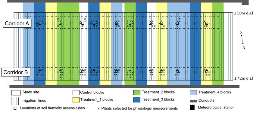
Forests 2020, 11, 88                                                                                                     4 of 15

end of each irrigation period, irrigation water was supplied for 10 min with Nutrifluid© NPK 12:6:6,
corresponding to 11.5 kg ha−1 week−1 . Nutrients supply did not vary among treatments. Plants were
irrigated overnight to allow rehydration when stomata are closed. Fertigation ended with the first
autumn rains on October 26th, lasting 21 weeks.

      Table 2. Irrigation treatments applied on the experimental plot in summer 2016, per week and
      total season.

                                                                                       Treatments
                   Period        Irrigation Parameters
                                                               Control       1         2         3          4
                                 Total volume (mm) *              **        1.88      3.12      4.38       5.62
                  Weekly            Frequency (x)                 **         3         3         3          3
                                Drip fertilization (min.)         **         30        30        30         30
               Total season           Volume (mm)                 21       39.48     65.52     91.98     118.02
      * The increase in water volume was obtained by increasing each irrigation period. ** control was irrigated 3 days by
      month (every four weeks).

2.5. Data Collection

2.5.1. Meteorological Data
      A portable meteorological station with data logger placed near the center of the experimental plot
(Figure 1) permanently gathered and store information every ten minutes about air temperature (Ta
in ◦ C), rainfall (mm), relative air humidity (raH in %), air pressure (EA in mbar), wind direction and
velocity (ms−1 ). Air vapor pressure deficit (VPD in Pa) was calculated with the following equation [19]:

                       VPD = Saturated Vapor Pressure (ES) − Actual Vapor Pressure (EA)                                      (1)

where ES = 0.6108 EXP ((17.27 × Ta)/(Ta + 237.3)) and EA = (raH × ES)/100

2.5.2. Soil Moisture
     Soil water profile was monitored at four locations per treatment along two elevations, totaling
20 locations (Figure 1): half of the monitoring points were at 47 m a.s.l and the remaining at 43 m a.s.l.
Specific tubes for measuring soil water profile were installed between the plant and the irrigation tube
30 cm apart. Volumetric water content (%) was measured weekly in each location at six depths down
to 100 cm with a Profile probe (PR2, Delta-T Devices). Between measurements, soil profile equipment
was permanently installed in the field and locations were changed every 15 days.
     As irrigation tubes were placed 40 cm deep, soil moisture measurements were grouped into two
classes: sub-surface (0 down to 40 cm) and deep (40 cm to 100 cm deep) soil water storage (mm),
according to the following equations:

          Sub-surface water storage (mm) = (θ0.1 × 0.15 m + θ0.2 × 0.10 m + θ0.3 × 0.10 m) × CF                              (2)

                 Deepwater storage (mm) = (θ0.4 × 0.20 m + θ0.6 × 0.25 m + θ1.0 × 0.20) × CF                                 (3)

where: θa is the volumetric water content by depth (a in meters) and CF is the conversion factor of
water volume (m3 m−3 to mm m−2 ) = 10

2.5.3. Dendrometric Measurements
     All plants were measured before and after treatments in February 2016 and 2017 (previously
to the spring growing season). At the same time, plants’ vitality was accessed visually (defoliation
and drying). Stem diameter at the base (Db) was measured with millimeter-precision using caliper
and total height (tH) was centimeter-accurate with a measuring tape. Plants’ crown area was not
Forests 2020, 11, 88 5 of 15
measured as most plants had no apical dominance yet. Relative growth was calculated using the
following equations:
Relative diameter growth: Rg.Db2016 (%) = (Db2017 − Db2016)/Db2016 × 100 (4)
Relative height growth: Rg.tH2016 (%) = (tH2017 − tH2016)/tH2016 × 100 (5)
2.5.4. Stomatal Conductance
Plants located at corridors A or B near soil moisture tubes (Figure 1) were selected for physiological
measurements. From 7th July until 8th September 2016 stomatal conductance (mmol m−2 s−1 ) was
measured weekly with a portable diffusion porometer (AP4, Delta-T Devices Ltd., Cambridge, UK) in a
total sample of 147 plants. Four fully expanded, south-oriented/sun-exposed leaves of the current-year
spring flushing with appropriate size and smooth were selected from each plant. On each day of
measurements, stomatal conductance was monitored in about 55 plants between 10:00 h and 16:00 h.
2.5.5. Statistical Analysis
Statistical analysis were made using the SPSS v.22 software package (IBM Corp., Armonk, NY,
USA). Before statistical modeling, all variables were graphically explored regarding distribution
patterns and outliers. No transformation was required and values that clearly corresponded to errors
in measurements were removed. Analysis of Variance (ANOVA) was performed for each block to
compare dendrometric parameters (diameter, height or relative growth) between plants from the
center and the margin. As the results were not statistically different, all the plants were included
in the following dendrometric models. A General Linear Mixed model was applied to analyze:
(1) if deepwater storage with repeated measurements over the summer was related to treatments,
to elevation (two classes), and to time (day of measurement); (2) If stomatal conductance, grouped by
soil moisture locations and with repeated measurements over the summer was related to treatments,
to elevation (two classes), to deepwater storage, to hour of the day, to time (day of measurement) and
to several meteorological variables (air temperature, relative air humidity, calculated air vapor pressure
deficit, wind velocity); Interactions were tested; (3) If each dendrometric parameter (diameter or height,
or their relative growth), grouped by plants within blocks was related to the initial dendrometric
parameter, to the distance to the stream, to elevation, or to treatments. In all the mixed models,
non-significant independent variables were removed and, additionally, interaction between significant
variables was tested. Several covariance structures were tested, selecting the one that best fit the
data according to the information criteria. If the variance related to the random variables (block or
locations) was not statistically significant, a model was tested without grouping plants within blocks
or locations. Estimated marginal means of fitted model were requested, comparing the main effects
with all the available methods (Least Significance Difference, Bonferroni, and Sidak). When applying
General Lineal Models (when subjects were not grouped and there was no repeated measurements)
contrast tests were performed. Treatment variable was reclassified according to the significance of the
estimates of fixed effects, grouping those that were not statistically different and a new mixed model
was performed.
3. Results
3.1. Meteorology
The ombrothermic diagram (Figure 2) indicates monthly precipitation/irrigation and mean
temperature in the study field since the first summer after planting. During the four-month irrigation
treatments, the daily temperature averaged 20.9 ± 3.5 ◦ C and total precipitation was only 42 mm.
Irrigation provided monthly water inputs ranging from 4 mm (control) to 24.4 mm (treatment 4).
The month before the treatments was the wettest of 2016, where precipitation exceeded 120 mm.Forests 2020, 11, 88 6 of 15
Forests
Forests 2020,
2020, 11,
11, xx FOR
FOR PEER
PEER REVIEW
REVIEW 66 of
of 15
15
Figure
Figure Ombrothermic chart of
2. Ombrothermic of monthly rainfall
rainfall and mean
mean temperature that
that occurred in
in the
Figure 2.
2. Ombrothermic chartchart of monthly
monthly rainfall and
and mean temperature
temperature that occurred
occurred in the
the
experimental
experimental plot since
plot since planting,
planting, including
including monthly
monthly irrigation
irrigation water
water inputs
inputs per
per treatment.
treatment. Control
Control
experimental plot since planting, including monthly irrigation water inputs per treatment. Control
received
received survival irrigation.
received survival
survival irrigation.
irrigation.
3.2. Soil Moisture
3.2.
3.2. Soil
Soil Moisture
Moisture
During 2016, surface soil moisture (above irrigation tubes) ranged from ≈0% to 13%; Changes in
During
During 2016,
2016, surface
surface soil
soil moisture
moisture (above
(above irrigation
irrigation tubes)
tubes) ranged from
from ≈0%
≈0% to
to 13%;
13%; Changes
Changes in
moisture were closely associated with daily precipitation (Figureranged
3). in
moisture were closely associated with daily precipitation (Figure
moisture were closely associated with daily precipitation (Figure 3). 3).
Figure 3.3.Average (lines) andand
standard deviation (vertical lines) of instantaneous soil moisture measured
Figure 3. Average
Average (lines)
(lines) and standard
standard deviation
deviation (vertical
(vertical lines)
lines) of
of instantaneous
instantaneous soil
soil moisture
moisture
at six depths
measured in all the locations from the experimental plot, and daily precipitation (black bars) during
measured at six depths in all the locations from the experimental plot, and daily precipitation (black
at six depths in all the locations from the experimental plot, and daily precipitation (black
summer
bars) 2016.summer 2016.
during
bars) during summer 2016.
In
In deep layers (60 and
and 100 cm)
cm) soil moisture
moisture fluctuated between 4% and 46%. Water
Water soil storage
storage
In deep
deep layers
layers (60
(60 and 100
100 cm) soil
soil moisture fluctuated
fluctuated between
between 4% 4% and
and 46%.
46%. Water soil
soil storage
reached
reached 116.3 ± 18.8 mm inin spring and
and slowly halved
halved throughout the the summer (p (p < 0.001, Table
Table A1)
reached 116.3
116.3 ±± 18.8
18.8 mm
mm in spring
spring and slowly
slowly halved throughout
throughout the summer
summer (pForests 2020, 11, 88 7 of 15
despite irrigation treatments. The upper part of the experimental field presented lower values for
deepwater storage (28–86 mm) than down the hill ((41–142 mm), p < 0.001). However, when soil was
saturated (June) no differences between elevations were observed (t: −1.77, p = 0.103). There was no
significant relationship between irrigation treatments and deep soil water storage (p = 0.057, Table A1).
Additionally, continuous measurements at several locations showed no variation in soil water profile
after or during the irrigation periods (data not shown).
3.3. Functional Parameters: Stomatal Conductance
Stomatal conductance varied between 34 mmol m−2 s−1 and 449 mmol m−2 s−1 , with mean +
standard deviation = 191 ± 72 mmol m−2 s−1 . Using the mixed models’ procedure (that considers
non-independence of the data measured on the same plant on different days and plants grouped by
location) there was no statistical significance between treatments and stomatal conductance (p > 0.05).
However, since the variance between locations did not explain the observed variance (p = 0.092;
Table A2), the random grouping within locations was removed. Standard errors and confidence
intervals decreased and treatments were statistically significant (p = 0.001). Stomatal conductance
in control and treatment 1 were significantly lower than in the remaining treatments which, in turn,
were similar between them (Table A3). Therefore, treatments were reclassified and the first model
was again performed. A statistically significant relationship between stomatal conductance and
treatments was obtained with this model (Table 3). This physiological parameter was about 15%
lower in control and treatment 1 than in the remaining treatments (176.91 ± 6.32 mmol m−2 s−1 and
203.51 ± 5.53 mmol m−2 s−1 , respectively). Additionally, stomatal conductance tended to decrease over
the summer and was positively related to plants’ dimension (initial diameter at the base). Deepwater
storage was also associated with stomatal conductance: for each 1 mm increase in deepwater storage,
leaf stomatal conductance increased 1.4 mmol m−2 s−1 . Meteorological data and hour of the day were
not associated with this physiological parameter and removed from the model. Regarding hour of the
day, graphical analysis showed that stomatal conductance displayed little variation between 10:00 h
and 16:00 h.
Table 3. Independent fixed effects of the generalized linear mixed model (GLMM) with two treatment
classes on the stomatal conductance (mmol m−2 s−1 ) measured in 147 plants grouped by “location” as a
random effect with a first-order autoregressive structure, in the experimental plot during the irrigation
period (summer 2016).
95% Confidence Interval
Parameter Estimate S.E. t Value
p Value Lower Upper
Intercept 116.46 25.04 4.65Forests 2020, 11, 88 8 of 15
Forests 2020, 11, x FOR PEER REVIEW 8 of 15
Forests 2020, 11, x FOR PEER REVIEW 8 of 15
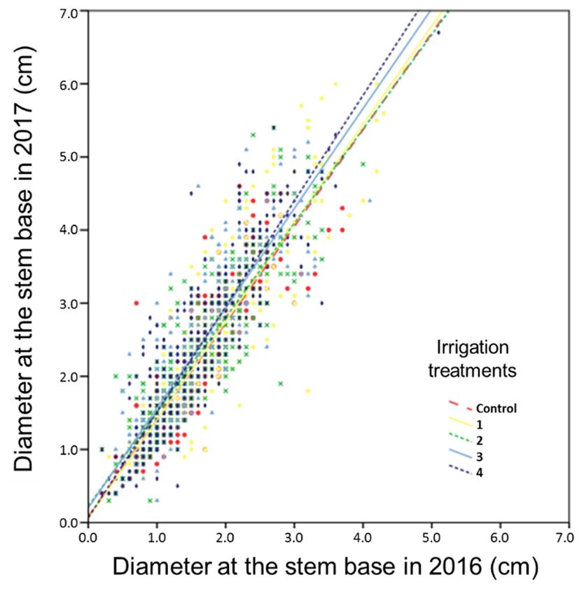
Figure 4. Linear
Figure relationship
4. Linear between
relationship betweeninitial
initial(2016) andfinal
(2016) and final(2017)
(2017) diameter
diameter at the
at the base,
base, separated
separated by by
irrigation treatments.
irrigation treatments.
Figure 4. Linear relationship between initial (2016) and final (2017) diameter at the base, separated by
irrigation treatments.
The Theresults were
results werequite
quitesimilar
similar for relativediameter
for relative diameter growth
growth (F =(F = 3.23,
3.23, p = However,
p = 0.047). 0.047). However,
this
this parameter
parameter isis dimensionless
dimensionless and,
and, therefore,
therefore, a a
better better
growth growth
indicatorindicator
of plants of plants
with
The results were quite similar for relative diameter growth (F = 3.23, p = 0.047). However, this with
disparate disparate
initial
sizes. In In
initialparameter
sizes. addition,
addition,
is using relative
using
dimensionless increments
relative
and, arather
increments
therefore, than
betterratherabsolute
growththan values
absolute
indicator ofallowed measuring
valueswith
plants allowed theinitial
effect the
measuring
disparate
of the
effectsizes.
of the initial
In initialvalues
addition, valueson growth.
usingon Since
growth.
relative the random
Since the
increments variable
random
rather blocks
variable
than absolute was not
blocks
values significant
was not
allowed (Wald Z:
significant
measuring 1.26, p
(Wald
the effect Z:
= 0.210),
p =the
1.26, of a general
initialavalues
0.210), linear
general model
on growth. was applied
Since the
linear model wasrandom without
applied grouping
variable
withoutblocksthe plants
was not the
grouping into blocks.
significant
plants (WaldIn this model
Z: 1.26, In
into blocks. p this
model =(Table
0.210),A4),general
(TableaA4),
irrigation treatments
linear
irrigation model were
was
treatments
more without
applied associated with increments
grouping
were more associated the
withplants (F = 7.15,
into
increments
p < In
blocks. 0.001)
(F = 7.15,
after a
p < 0.001)
this model
reduction in the standard errors and confidence intervals, but the tendency remained the same
after (Table A4), irrigation
a reduction treatments
in the standard wereand
errors more associatedintervals,
confidence with increments
but the(Ftendency
= 7.15, p remained
< 0.001) aftertheasame
(Figure 5). Treatment contrasts of the last model reinforce the results (Table
reduction in the standard errors and confidence intervals, but the tendency remained the same A4a).
(Figure 5). Treatment contrasts of the last model reinforce the results (Table A4a).
(Figure 5). Treatment contrasts of the last model reinforce the results (Table A4a).
Figure 5. G.L.M.M. estimated marginal means of the relative diameter growth at the base (%) by
Figure 5. G.L.M.M.
irrigation estimated
treatments, marginal
with plants means
grouped of the relative
or not diameterletters
growth at the base (%) by
Figure 5. G.L.M.M. estimated marginal means ofwithin blocks.diameter
the relative Different
growth at denote statistically
the base (%) by
irrigation treatments, with
significanttreatments, plants
differenceswith grouped
at theplants
5% level or
without not within
grouping blocks. Different letters denote statistically
irrigation grouped or not withinplants
blocks.within blocks
Different as a random
letters factor.
denote statistically
significant differences at the 5% level without grouping plants within blocks as a random factor.
significant differences at the 5% level without grouping plants within blocks as a random factor.
Considering the significant differences between treatments, the inflection point was on treatment
2 corresponding to an average increment of 47% (Figure 5). Again, control and treatment 1 were
different from the remaining treatments (Table A4) and, similar to stomatal conductance models,Forests 2020, 11, 88 9 of 15
treatments could be classified into two classes. The new mixed model with plants within blocks
showed that the increase in diameter was ≈10% inferior in plants from control and treatment 1 (Table 4).
Additionally, the relative increment was lower in larger plants (t = −4.965, p < 0.001). Distance to
the stream was also negatively associated with diameter growth, though elevation was not (p > 0.05,
removed from the model). Nevertheless, one should note that the variance in residuals was very large
(Table A5). In regards to total height, average + S.D. was 66.6 ± 35.7 cm, relative increment was ≈22%
and treatments were not significant (p > 0.05). Initial height values negatively influenced the relative
growth (t = −11.171, p < 0.001) and distance to the stream showed a stronger negative relation with
height than with relative diameter growth (t = −6.857, p < 0.001).
Table 4. Generalized linear mixed model (GLMM) Estimates of the Independent fixed effects on the
relative diameter growth at the base (%)”, grouped by plants within blocks as a random effect with a
first-order autoregressive structure and combining treatments into two classes, in the experimental plot
after the irrigation period.
95% Confidence Interval
Parameter Estimate S.E t Value
p Value Lower Upper
Intercept 78.70 7.85 10.02Forests 2020, 11, 88 10 of 15 inputs. In fact, continuous measurements also failed to distinguish water inputs from irrigation, confirming that the wet-bulb did not extend horizontally up to 30 cm. This parameter was not useful for a future irrigation water management in the sandy soils of the experimental site, however, other information was possible to obtain from soil water profile. Both soil analysis and soil water monitoring allowed inferring the soil water capacity of the experimental plot: measurements performed after rainy periods indicated that field capacity down to 1 m varied slightly across all profiles. On the other hand, measurements performed in summer highlighted two conditions: (1) surface moisture (0–30 cm, Figure 3) was below the permanent wilting point for this soil type (
Forests 2020, 11, 88                                                                                             11 of 15

treatments can be associated with the reduced apical dominance observed in the plants at the study
site. This condition may change over time.

5. Conclusions
      Field experiments usually pose more challenges, but the results have better external validity,
and are applicable to natural conditions. Despite the constraints related to soil conditions, particularly
the low soil water retention, irrigation was significantly associated with the plants’ functional-structural
response. A 3-fold increase in water corresponded to a 15% increase in stomatal conductance and a 10%
increase in stem diameter. Hence, stomatal conductance may be the link between water availability and
plant growth in the following studies. These results are promising in the analysis of the best irrigation
regime for cork oaks under natural conditions. Plant needs and their resource use efficiency change
over time, as well as abiotic factors such as meteorological conditions. Therefore, the study should be a
long-term project in order to meet to the main objective of the best irrigation regime for all scenarios.

Author Contributions: Conceptualization, M.V., J.M.B. and N.A.R.; Formal analysis, C.C.-A.; Funding acquisition,
N.A.R.; Investigation, C.C.-A. and C.D.; Methodology, M.V., J.M.B. and N.A.R.; Supervision, N.A.R.; Validation,
M.V., J.M.B. and N.A.R.; Writing-original draft, C.C.-A.; Writing-review & editing, C.C.-A., C.D., M.V. and J.M.B.
All authors have read and agreed to the published version of the manuscript.
Funding: This research was funded by “Medida 4.1—Cooperação para a Inovação/ProDeR 52131
and 52132” REGASUBER: “Cork oaks (Quercus suber) under intensive production and fertigation”,
by PDR2020-101-FEADER-031427 “GO-RegaCork”, and by National Funds through FCT—Foundation for
Science and Technology under the Projects UID/AGR/00115/2019 and UIDB/05183/2020, C.C.A. received a master
grant “BI_Mestre_UEVORA_ICAAM_PRODER_52132”.
Acknowledgments: We are thankful to Fruticor and to Amorim Florestal for the field and logistic support.
Conflicts of Interest: The authors declare no conflict of interest. The funders had no role in the design of the
study; in the collection, analyses, or interpretation of data; in the writing of the manuscript, or in the decision to
publish the results.

Appendix A

      Table A1. Independent fixed effects of the General Linear Mixed Model applied to the dependent
      variable “deepwater storage” in 20 locations of the experimental field during the irrigation period.

                                   Parameters            F Value     df1     df2      p Value
                                Corrected model           5.14        6      214
Forests 2020, 11, 88 12 of 15
Table A3. Generalized linear mixed model (G.L.M.M.) estimates of covariance parameters on the
stomatal conductance measured in 147 plants subjected to irrigation treatments, NOT grouped by
“location”, in the experimental plot during the irrigation period (Summer 2016).
95% Confidence Interval
Parameter Estimate S.E. t Value
p Value Lower Upper
Intercept 183.76 17.25 10.65Forests 2020, 11, 88 13 of 15
Table A5. Generalized linear mixed model (GLMM) estimates of the covariance parameters on the
relative diameter growth at the base (%), grouped by plants within blocks as a random effect with a
first−order autoregressive structure and combining treatments into two classes, in the experimental
plot after the irrigation period.
95% Confidence Interval
Parameter Estimate S.E Wald Z p Value
Lower Upper
Residual 1683.86 59.69 28.21Forests 2020, 11, 88 14 of 15
16. Pinto, C.A.; David, J.S.; Cochard, H.; Caldeira, M.C.; Henriques, M.O.; Quilhó, T.; David, T.S. Drought-induced
embolism in current-year shoots of two Mediterranean evergreen oaks. For. Ecol. Manag. 2012, 285, 1–10.
[CrossRef]
17. ICNF. 5◦ Inventário Florestal Nacional; Instituto da Conservação da Natureza e das Florestas: Lisboa, Portugal,
2010. Available online: http://www2.icnf.pt/portal/florestas/ifn/ifn5/rel-fin (accessed on 9 October 2018).
18. Dinis, C.; Camilo-Alves, C.; Vaz, M.; Almeida Ribeiro, N. 2018. Ripping Plantation Lines Improves Deep
Root Development of Container-Grown Cork-Oak Seedlings; World Congress SilvoPastoral Systems: Evora,
Portugal, 2016.
19. Tetens, O. Uber einige meteorologische Begriffe. Z. Geophys. 1930, 6, 297–309.
20. Campbell, G.S.; Norman, J.M. An Introduction to Environmental Biophysics, 2nd ed.; Springer Science &
Business Media: New York, NY, USA, 2012; pp. 129–144.
21. Hao, A.; Marui, A.; Haraguchi, T. Estimation of Wet-bulb Formation in Various Soil during Drip Irrigation.
J. Fac. Agric. Kyushu Univ. 2007, 52, 187–193.
22. Saxton, K.E.; Rawls, W.J. Soil water characteristic estimates by texture and organic matter for hydrologic
solutions. Soil Sci. Soc. Am. J. 2006, 70, 1569–1578. [CrossRef]
23. Farquhar, G.D.; Sharkey, T.D. Stomatal conductance and photosynthesis. Annu. Rev. Plant Physiol. 1982, 33,
317–345. [CrossRef]
24. Jones, H.G. Plant water relations and implications for irrigation scheduling. Acta Hortic. 1990, 278, 67–76.
[CrossRef]
25. Dolman, A.J.; Van Den Burg, G.J. Stomatal behaviour in an oak canopy. Agric. For. Meteorol. 1988, 43, 99–108.
[CrossRef]
26. Matsumoto, K.; Ohta, T.; Tanaka, T. Dependence of stomatal conductance on leaf chlorophyll concentration
and meteorological variables. Agric. For. Meteorol. 2005, 132, 44–57. [CrossRef]
27. Vialet-Chabrand, S.; Dreyer, E.; Brendel, O. Performance of a new dynamic model for predicting diurnal
time courses of stomatal conductance at the leaf level. Plant Cell Environ. 2013, 36, 1529–1546. [CrossRef]
[PubMed]
28. Urban, J.; Ingwers, M.W.; McGuire, M.A.; Teskey, R.O. Increase in leaf temperature opens stomata and
decouples net photosynthesis from stomatal conductance in Pinus taeda and Populus deltoides x nigra. J. Exp.
Bot. 2017, 68, 1757–1767. [CrossRef] [PubMed]
29. Dinis, C. Cork Oak (Quercus suber L.) Root System: A Structural-Functional 3D Approach. Ph.D. Thesis,
Evora University, Evora, Portugal, 2014.
30. Puértolas, J.; Pardos, M.; Jiménez, M.D.; Aranda, I.; Pardos, J.A. Interactive responses of Quercus suber L.
seedlings to light and mild water stress: Effects on morphology and gas exchange traits. Ann. For. Sci. 2008,
65, 611. [CrossRef]
31. Schmidt, M.W.T.; Schreiber, D.; Correia, A.; Ribeiro, N.; Surový, P.; Otieno, D.; Tenhunen, J.; Pereira, J.S. Sap
flow in cork oak trees at two contrasting sites in portugal. Acta Hortic. 2009, 846, 345–352. [CrossRef]
32. Rzigui, T.; Jazzar, L.; Baaziz Khaoula, B.; Fkiri, S.; Nasr, Z. Drought tolerance in cork oak is associated with
low leaf stomatal and hydraulic conductances. iForest Biogeosci. For. 2018, 11, 728. [CrossRef]
33. Aranda, I.; Castro, L.; Pardos, M.; Gil, L.; Pardos, J.A. Effects of the interaction between drought and shade
on water relations, gas exchange and morphological traits in cork oak (Quercus suber L.) seedlings. For. Ecol.
Manage. 2005, 210, 117–129. [CrossRef]
34. Merouani, H.; Branco, C.; Almeida, M.H.; Pereira, J.S. Effects of acorn storage duration and parental tree on
emergence and physiological status of Cork oak (Quercus suber L) seedlings. Ann. For. Sci. 2001, 58, 543–554.
[CrossRef]
35. Branco, M.; Branco, C.; Merouani, H.; Almeida, M.H. Germination success, survival and seedling vigour of
Quercus suber acorns in relation to insect damage. For. Ecol. Manag. 2002, 166, 159–164. [CrossRef]
36. Pons, J.; Pausas, J.G. Oak regeneration in heterogeneous landscapes: The case of fragmented Quercus suber
forests in the eastern Iberian Peninsula. For. Ecol. Manag. 2006, 231, 196–204. [CrossRef]
37. Trubat, R.; Cortina, J.; Vilagrosa, A. Nursery fertilization affects seedling traits but not field performance in
Quercus suber L. J. Arid Environ. 2010, 74, 491–497. [CrossRef]Forests 2020, 11, 88 15 of 15
38. Ribeiro, N.A.; Surový, P. Growth modeling in complex forest systems: CORKFITS a tree spatial growth
model for cork oak woodlands. Formath 2011, 10, 263–278. [CrossRef]
39. Tenhunen, J.; Geyer, R.; Carreiras, J.M.B.; Ribeiro, N.A.; Dinh, N.Q.; Otieno, D.; Pereira, J.S. Simulating
function and vulnerability of cork oak woodland ecosystems. In Cork Oak Woodlands on the Edge: Ecology,
Adaptive Management, and Restoration; Pereira, J.S., Pausas, J.G., Aronson, J., Eds.; Society for Ecological
Restoration International; Island Press: Washington, DC, USA, 2008; pp. 227–234.
© 2020 by the authors. Licensee MDPI, Basel, Switzerland. This article is an open access
article distributed under the terms and conditions of the Creative Commons Attribution
(CC BY) license (http://creativecommons.org/licenses/by/4.0/).You can also read