Going Deep: Graph Convolutional Ladder-Shape Networks - Shirui Pan
←
→
Page content transcription
If your browser does not render page correctly, please read the page content below
Going Deep: Graph Convolutional Ladder-Shape Networks

            Ruiqi Hu,1 Shirui Pan,2 Guodong Long,1 Qinghua Lu,3 Liming Zhu,3 Jing Jiang1
                          1
                              Centre for Artificial Intelligence, University of Technology Sydney, Australia
                                               2
                                                 Faculty of IT, Monash University, Australia
                                                              3
                                                                Data61, CSIRO
                               {ruiqi.hu, guodong.long, jing.jiang}@uts.edu.au, shirui.pan@monash.edu
                                                 {qinghua.lu, liming.zhu}@data61.csiro.au

                              Abstract                                 Zhang et al. 2016) and image classification(Liu et al. 2019b;
                                                                       2019a)).
  Neighborhood aggregation algorithms like spectral graph
  convolutional networks (GCNs) formulate graph convolu-                  There has recently been a rise in interest in leveraging
  tions as a symmetric Laplacian smoothing operation to ag-            embedding methods or deep learning algorithms for graphs.
  gregate the feature information of one node with that of its         Many probabilistic models (Grover and Leskovec 2016;
  neighbors. While they have achieved great success in semi-           Tang et al. 2015) or matrix factorization-based works (Cao,
  supervised node classification on graphs, current approaches         Lu, and Xu 2015; Wang et al. 2017) aim to capture the pat-
  suffer from the over-smoothing problem when the depth of             terns (walks) with neighborhood connections and the first or
  the neural networks increases, which always leads to a notice-       second order proximities from a graph, and to encode the
  able degradation of performance. To solve this problem, we
  present graph convolutional ladder-shape networks (GCLN),
                                                                       graph into a low-dimensional, compact vector space. The
  a novel graph neural network architecture that transmits mes-        well-learned embedding can be directly analyzed by conven-
  sages from shallow layers to deeper layers to overcome the           tional machine learning approaches. These methods exploit
  over-smoothing problem and dramatically extend the scale             and preserve the topological characteristics and lose sight of
  of the neural networks with improved performance. We have            the contextual features of the nodes in the graph.
  validated the effectiveness of proposed GCLN at a node-wise             Other methods simultaneously consider structural char-
  level with a semi-supervised task (node classification) and an       acteristics and node features to learn a robust embedding
  unsupervised task (node clustering), and at a graph-wise level
  with graph classification by applying a differentiable pooling
                                                                       of the graph. Examples in this category include content
  operation. The proposed GCLN outperforms original GCNs,              enhanced network embedding methods and neighborhood
  deep GCNs and other state-of-the-art GCN-based models for            aggregation (or message passing) algorithms. Content en-
  all three tasks, which were designed from various perspec-           hanced methods associate text features with the representa-
  tives on six real-world benchmark data sets.                         tion architectures, examples like TADW (Yang et al. 2015)
                                                                       which incorporates the feature information into network
                                                                       representation under a matrix factorization framework and
                       Introduction                                    TriDNR (Pan et al. 2016) which trains a neural network ar-
Graphs are of the essence for constructing non-Euclidean               chitecture to capture both structural proximity and attribute
data and they are omnipresent in most areas. In the social             proximity from the attributed graph. Neighborhood aggre-
media industry, for instance, users, through their personal            gation algorithms (Dai et al. 2018; Li, Han, and Wu 2018;
profile information, are linked with and interact with other           Klicpera, Bojchevski, and Günnemann 2018), represented
users (e.g., friends, colleagues), and the entire social me-           as spectral graph convolutional networks (spectral GCNs)
dia network is modeled as an attributed graph for prod-                (Kipf and Welling 2016b), introduce the Laplacian smooth-
uct/friend/community recommendations (node clustering);                ing operation to propagate the attributes of a node over its
In medicine and pharmacology, molecules and chemical                   neighborhood. Spectral-based algorithms have commanded
bonds can be constructed as graphs to potentially discover             more attention among the aforementioned approaches due to
new drugs by identifying their bio-activities (node clas-              their significant improvements over semi-supervised tasks.
sification (Defferrard, Bresson, and Vandergheynst 2016;                  Spectral-based algorithms borrow the idea of filters from
Gilmer et al. 2017)); In academic citation networks, pa-               the graph signal processing domain to conduct the graph
pers are connected by their citations, and the titles, au-             convolution operation, which can also be interpreted as elim-
thors, venues and keywords form graph characteristics for              inating noises from graph signal. The major difference be-
automatic categorization (semi-supervised node classifica-             tween one type of spectral GCN and another lies in the de-
tion (Velickovic et al. 2017; Kipf and Welling 2016b;                  sign of the filter. Spectral CNNs (Bruna et al. 2013) formu-
Copyright © 2020, Association for the Advancement of Artificial        late the filter with a collection of learnable parameters to
Intelligence (www.aaai.org). All rights reserved.                      implement the convolution operation based on the spectrum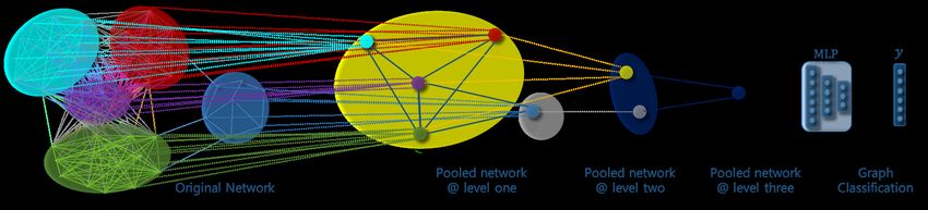
more than three convolutional layers) because of the over-
                                                                smoothing of features during the propagation procedure.
                                                                   To further extend GCLN to exploit the hierarchical em-
                                                                bedding information of graphs, we also fuse a differentiable
                                                                graph pooling module (Ying et al. 2018) with our frame-
                                                                work, so that GCLN can infer and aggregate the local topo-
                                                                logical structure as well as the coarse-grained topological
                                                                structure over graphs. We have not only evaluated the effec-
                                                                tiveness of GCLN with a semi-supervised task and unsuper-
                                                                vised task at the node-wise level, but have also conducted
Figure 1: Influence of the depth of graph convolutional net-    graph classification to validate its predictive performance at
works on semi-supervised node classification performance.       the graph-wise level.
When GCN goes deep (layer>3), its classification accuracy          Our main contributions are summarized as follows:
is decreased as the number of layers increases.                 • We propose a novel graph convolutional network symmet-
                                                                  rically constructed on one contracting and one expand-
                                                                  ing path with contextual feature channels, which dramat-
of the graph Laplacian. ChebNet (Defferrard, Bresson, and         ically extends the depth of spectral graph convolutional
Vandergheynst 2016) considers the filter as Chebyshev poly-       networks.
nomials of the diagonal matrix of eigenvalues, where the
Chebyshev polynomial is defined with a recursive formu-         • The proposed graph convolutional ladder-shape net-
lation. Spectral GCNs (Kipf and Welling 2016b) can be in-         work (GCLN) solves the problem of over-smoothed fea-
terpreted as the first order approximation of ChebNet, which      tures with many convolutional layers in neighborhood
assumes that the order of the polynomials of the Laplacian is     aggregation-based neural networks.
restricted to 1 while the maximum of the eigenvalues is re-     • Extensive experiments on semi-supervised and unsuper-
stricted to 2. Most recently, g-U-Nets (Gao and Ji 2019) at-      vised node-wise node level tasks, and a graph-wise task
tempts to generate the position information of selected nodes     compared with sufficient classical and state-of-the-art
by using proposed gPooling and gUnpool operations, so the         baselines demonstrate the effectiveness of GCLN.
classic computer vision methods can be applied in graphs
and increases the depth of the architecture. However, this                          Problem Definition
method heavily relays on the graph preprocessing and can
                                                                A graph is defined as G = {V, E}, where {vi }i=1,··· ,n ∈ V
be difficult to train for good performance.
                                                                represents all the nodes in a graph. ei,j = (vi , vj )i,j=1,··· ,n ∈
   The major problem with all the aforementioned algo-
                                                                E indicates the set of binary linkage relationships between
rithms is that the quality of the neighborhood aggrega-
                                                                two nodes, where ei,j = 1 if there is an edge between nodes
tion procedure inevitably declines in a deep neural net-
                                                                vi and vj , otherwise, ei,j = 0. An adjacency matrix A is used
work architecture that has many graph convolutional lay-
                                                                to mathematically present the topological information of the
ers (Klicpera, Bojchevski, and Günnemann 2018). The line
                                                                graph G, where each cell of the matrix A maps the corre-
chart (Fig.1) illustrates how the performance is degraded as
                                                                sponding edge information encoded in E. A feature matrix
the depth of the GCN model is increased. The main reason
                                                                X preserves the features xi ∈ X pertinent to the node vi .
for this problem is that Laplacian smoothing in these ag-
gregation (or propagation) schemes over-smooths the node        Node-wise Embedding Definition
features and renders the nodes from different clusters in-
                                                                Given G, the objective of graph neural networks is to embed
                                                                                                                   R
distinguishable (Xu et al. 2018). Explicitly, adding multiple
GCN layers is equivalent to repeatedly conducting a Lapla-      all the nodes V into a compact space Z ∈ n×d through
cian smoothing operation, and the features of neighboring       f : (A, X) 7−→ Z, where d, normally a smaller number, is
connected nodes in the graph will converge to the same val-     the dimension of the learned embedding. zi ∈ Z indicates
ues. In the case of spectral GCN, the features will converge    the encoded node vi with associated topological informa-
in proportion to the square root of the node degree (Li, Han,   tion from A and feature information from X. Ideally, nodes
and Wu 2018), which is the over-smoothing problem ad-           with similar characteristics are expected to remain close in
dressed in this paper.                                          the embedding space. With well-learned embedding Z of the
   In this paper, we propose a novel graph convolutional        graph G, the classical machine learning methods can be di-
architecture, graph convolutional ladder-shape networks         rectly applied for semi-supervised tasks like node classifica-
(GCLN), which is built upon one contracting path and            tion and unsupervised tasks like node clustering.
one expanding path with contextual feature channels. The
ladder-shape architecture allows the network to directly        Graph-wise Classification Definition
transmit and fuse the contextual information from the shal-     Given a set of aforementioned graphs G                   =
low layers to the deeper layers, which challenges the as-       {(G1 , y1 ), (G2 , y2 ), ..., (Gk , yk )} where Gk ∈ G with
sumption that neighborhood aggregation-based architec-          the corresponding labels yk ∈ Y, the purpose of graph-wise
tures can only be shallow networks (e.g., the GCN per-          tasks such as graph classification is to learn a mapping
formance will necessarily be degraded when there are            f : G 7−→ Y which assigns the given graphs to the labels.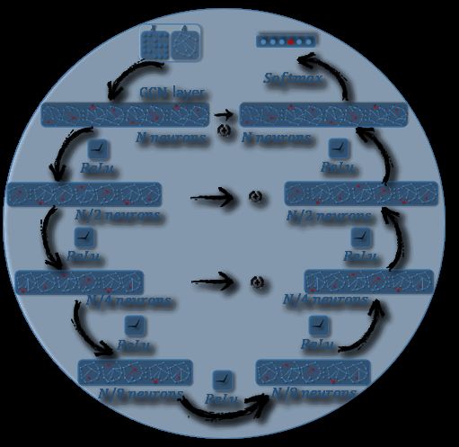
Each given graph is embedded into a low-dimensional The up-sampling path is also comprised of four similar
vector based on which the class label of the whole graph de-convolutional blocks and enables the model to simultane-
can be inferred. ously obtain accurate localization information and sufficient
contextual information from the down-sampling path.
Preliminaries The U-Net adequately and simultaneously exploits the
precise localization from the up-sampling path and the con-
The proposed GCLN is most related to two models: spec- textual information from the down-sampling path. The two
tral graph convolutional networks and u-shape networks. sources of information are correspondingly concatenated
We also employ the differentiable graph pooling module to through the feature channels during the training for bio-
graph-wisely validate the effectiveness of GCLN. We elab- medical image segmentation.
orate the details of these three models in this section.
Differentiable Graph Pooling
Graph Convolutional Networks
The differentiable graph pooling module (Ying et al. 2018) is
designed to enable graph neural networks to conduct predic-
tive tasks over graphs rather than over nodes of one graph.
Graph pooling is necessary for graph-wise tasks such as
graph classification, and the challenge of the pooling oper-
ation in the graph setting, compared to the computer vision
setting, is that unlike an image, a graph has no natural spatial
location and unified dimension.
The differentiable graph pooling module solves the afore-
mentioned challenges by learning a differentiable soft as-
Figure 2: The architecture of a typical spectral graph convo- signment at each layer of a GNN model, assigning nodes
lutional network. The performance of GCNs with more than to a set of clusters according to the learned representations.
two or three layers will dramatically drop as a result of the Thus, the pooling operation of each GNN layer coarsens the
over-smoothing problem. given graph iteratively and generates a hierarchical repre-
sentation of every input graph on completion of the entire
Standard graph convolutional networks (GCNs) (Kipf and training procedure.
Welling 2016b), as shown in Figure 2, comprise a two-layer
semi-supervised framework which propagates the features Graph Convolutional Ladder-shape Networks
of a node over its neighboring nodes. The objective of GCNs
is to learn a spectral function f (X, A) where the adjacency
matrix A represents the topological characteristics of the
graph and matrix X preserves the interdependence of the
nodes and features. The propagation rule is more likely to
represent each node in the graph by aggregating its neigh-
borhood with self-loops, and the output of the networks is
a normalized node-level representation (or graph embed-
ding), which represents each node with a low-dimensional
vector. Because the spectral function f (•) conducts the fea-
ture smoothing on the topological adjacent matrix A, the
networks can distribute the gradient through the supervised
error and learn the representation of both annotated and un-
labeled nodes.
U-Net
The U-Net (Ronneberger, Fischer, and Brox 2015) is an el-
egant U-shape fully convolutional network architecture de-
veloped for bio-medical image segmentation. The architec-
ture consists of two parts: the down-sampling path and the
up-sampling path.
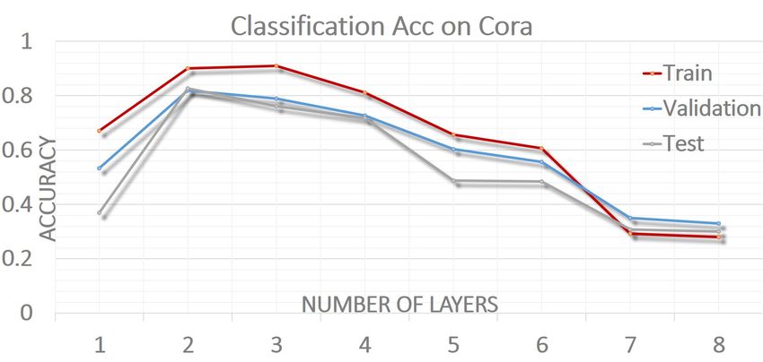
The down-sampling path is comprised of four blocks with Figure 3: Illustration of a graph convolutional ladder-shape
two convolutional layers and one max pooling (stride=2) networks (GCLNs). The network consists of two symmetric
layer for each block. At each step following the down- paths: a contracting path (left) and an expanding path (right).
sampling path, the number of feature channels is doubled. The contextual feature channels between the two paths are
The contracting path captures the contextual features from used to pass and fuse contextual information from the con-
the input image for segmentation and passes the features to tracting path to the location information from the expanding
the up-sampling path with skip connections. path in a simple but elegant operation.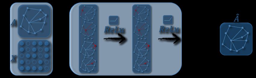
The proposed GCLN is a symmetric architecture con-            GCLN Contracting Path
structed of one contracting path and one expanding path
with GCN layers. Three contextual feature channels allow         The contracting path is a four-layer graph convolutional em-
the context features captured from the contracting path to       bedding architecture in which each layer halves the size (the
fuse with the localization information learned through the       number of neurons) of the previous layer. Each GCN layer
expanding path. Each layer is built with the spectral graph      conducts the graph convolution with Eq.(4), followed by the
convolution and there are eight GCN layers in total in the       ReLU activation and dropout.
proposed framework.                                                 The contracting path can be considered as the encoder part
                                                                 if GCLN is interpreted as an end-to-end encoder-decoder ar-
Graph Convolutional Operation                                    chitecture which encodes the topological characteristics and
The layers of GCLN are constructed on the first order ap-        features associated with each node into feature representa-
proximation of Chebyshev spectral CNNs. The graph con-           tions at multiple echelons. The contextual information of the
volution here can be defined by the normalized graph Lapla-      graph is captured through the contracting path and preserved
cian matrix :                                                    at each layer, and will be correspondingly transmitted to the
                                        1       1                expanding path via the contextual feature channels.
               gθ ⊗ x = θ0 Ix − θ1 D− 2 AD− 2 x,           (1)
                                         R
where gθ is the spectral filter, x ∈ n indicates the signal      GCLN Expanding Path
of the graph and ⊗ represents the convolution operator. Ix
is the identity matrix. D denotes the diagonal degree matrix     The expanding path mirrors the architecture of the contract-
of topological adjacency matrix A and θk is the Chebyshev        ing path with the arrangement of the layers reversed. Each
coefficients.                                                    layer doubles the number of neurons in the previous layer.
   Due to the condition of the first order approximation (Kipf   An element-wise summation operation is conducted to re-
and Welling 2016b), the Chebyshev coefficients are further       ceive and fuse the contextual information skipped from the
simplified with θ = θ1 = −θ0 , and the graph convolution is      contracting path as follows:
updated as:
                                     1      1
                                                                         Hlexpanding = summation Hl , H(L−l) .           (7)
               gθ ⊗ x = θ I + D− 2 AD− 2 x,                (2)
The convolution matrix is normalized through:                    where Hl is the latent representation from the lth layer and
                                              1    1             L is the number of graph convolutional layers. For the ex-
                    1      1
            I + D− 2 AD− 2 7−→ I + D e− 2 A
                                          eDe− 2        (3)
             P e                                                 periments described in this paper, L = 8.
where D = j Aij and A = A + I.
       e                 e                                          The contextual feature channels allow the network to go
   Adopting the definition of graph convolution, given a         deeper and to fuse the contextual features from the contract-
graph signal with m feature channels (e.g., X ∈ n×m , mR         ing side with the up-convolutional features from the expan-
features associated with each node), the layer-wise propa-       sive side. This summation enables representations to be bet-
gation rule of the spectral graph convolutional networks is      ter localized and obtained following many convolutions. The
defined as:                                                      indistinguishable features of nodes caused by repetitively
                               1         1
                                                                conducting a symmetrically normalized Laplacian smooth-
                        e− 2 A
             H(l+1) = ϕ D    eDe − 2 Hl Wl .               (4)   ing operation are directly characterized and enhanced, en-
                                                                 abling them to merge with the contextual features from the
where H0 = X and Hl is the activation from the lth GCN           contracting path. As a result, the over-smoothing problem of
layer. Wl is the trainable weight matrix and ϕ is the activa-    neighborhood aggregation-based algorithms is overcome.
tion function such as ReLU (•) and Linear(•).                       A softmax activation takes the output from the last graph
   For semi-supervised multi-class classification, the soft-     convolutional layer to conduct the semi-supervised node
max activation function is applied, row-wisely, to the final     classification with Eq.(5) and Eq.(6).
embedding of the graph. The form of the classifier is defined
as follows:                                                  Algorithm for GCLN
        C = softmax ÂReLU ÂXW(l−1) Wl .                  (5)
                                                                    The pseudo-code of GCLN is described in Algorithm 1.
               − 21   − 12                                       Step 2 walks through the contracting path and collects the
where  = D  e A  eDe    and Wl is the weight matrix be-        contextual information of the graph layer by layer, while
tween the last GCN-layer and the output layer.                   Steps 3 and 4 lead the network to go deep along the expan-
  The node classification loss function is written with cross-   sive path and fuse the corresponding contextual information
entropy error as follows:                                        via the feature channels. Steps 5 and 6 conduct the semi-
                          F
                         XX                                      supervised node classification and update the network.
                  L :=              Yif ln Cif .           (6)      In particular, the input for each graph convolution layer in
                         i∈Vl f=1                                the expanding path is the corresponding result of the sum-
where Vl denotes the set of annotated nodes and F is the         mation, rather than the direct latent matrix Hexp .
number of classes. Yif is the label indicator matrix mapping        Fig. 3 demonstrates the construction of the proposed
the predicted nodes.                                             GCLN.
Figure 4: Illustration of differentiable graph pooling procedure. At each hierarchical layer, the embeddings of nodes are learned
and obtained through a GCN layer, after which the nodes are clustered according to the learned embeddings into the coarsened
graph for another GCN layer. The process is iterated for l layers and the final output is used for the graph classification task.
Algorithm 1 Graph Convolutional Ladder-Shape Networks for Experiments
Node Classification
In this section, we set up the experiments compared to 15
Require:
G = {V, E}: a graph with nodes and edges;
classical and state-of-the-art methods to demonstrate the
X: the feature matrix; solid performance of GCLN on graph node classification.
T : the number of iterations; The experiments with 8-layer GCN and GAT validate the
o: the number of the neurons in the first convolution layer; existence of the over-smoothing problem and demonstrate
Ensure: o is divisible by 8. that GCLN is the solution to the problem. The contrast ex-
1: for iterator = 1,2,3, · · · · · · , T do periments compared residual GCN and GAT to illustrate that
2: Generate latent matrix H via Eq.(4) passing contracting residual connection cannot effectively ameliorate the prob-
path; lem. We also reveal the effectiveness of GCLN on unsuper-
3: Generate direct latent matrix Hexp via Eq.(4) passing ex- vised learning tasks with clustering experiments compared
panding path; to 16 peers. In addition, GCLN proves its predictive capabil-
4: Conduct corresponding summation via Eq.(7) with H and
Hexp ;
ity with the differentiable graph pooling module on graph-
5: Get the prediction results via Eq.(5) wise tasks such as graph classification.
6: Update the model with the loss computed via Eq.(6);
7: end for Data Sets
We conducted the experiments using three real-world bib-
liographic data sets: Cora, Citeseer and Pubmed (Sen et al.
Extension - GCLN with Differentiable Pooling 2008) and the details of the data set statistics are summa-
To extend GCLN for the graph-wise task, we have added rized in Table 1. The data sets are used for both node-wise
a differentiable pooling layer behind each GCN layer and classification and clustering.
taken the output from the last layer for graph classification.
The differentiable graph pooling formulates a general recipe Node Classification
for hierarchically pooling nodes across a set of graphs by We conducted node classification to validate the effective-
generating a cluster assignment matrix S over the nodes ness of GCLN on node-wise semi-supervised tasks.
leveraging the output of each GCN layer. The cluster ma-
trix S on layer l is computed as follows: Baseline Algorithms GCLN is compared with Classic
methods and GCN-based algorithms such as Chebyshev
S (l) = sof tmax GCN A(l) , X(l) . (8) (Defferrard, Bresson, and Vandergheynst 2016), GCN (Kipf
where GCN(A, X) is the graph convolutional operation and Welling 2016b), GraphInfoMax (Veličković et al. 2018),
elaborated in the last subsection and the softmax function LGCN (Gao, Wang, and Ji 2018), StoGCN (Chen, Zhu,
is row-wisely conducted. and Song 2018), DualGCN (Zhuang and Ma 2018), GAT
With cluster assignment matrix S, the differentiable pool- (Velickovic et al. 2017), and g-U-Nets (Gao and Ji 2019).
ing layer coarsens the given graph, generating a new adja- Node Classification Setup We used an eight GCN-layer
cency matrix A(l+1) and a new matrix X(l+1) by applying GCLN (except for the input layer and the layer with soft-
the following equations: max) to conduct all the experiments. The first layer consists
T
X(l+1) = S (l) Hl ∈ Rn l+1 ×d
. (9) of 64 neurons and each following layer in the contracting
path halves the number of neurons in the previous layer. Be-
A(l+1) = S (l) Al S (l) ∈ Rn
T
l+1 ×nl+1
. (10) cause of the symmetric architecture of GCLN, the first layer
(l+1) (l+1)
The generated A and X will be processed into the in the expanding path starts with 8 neurons and each subse-
next GCN layer. quent layer doubles the number of neurons, until 64 neurons
Fig. 4 illustrates the general process of the differentiable are found in the last layer. 0.9 dropout and the ReLU acti-
graph pooling. vation function were applied after every graph convolutionalTable 1: Datasets for Node Classification and Clustering
# Nodes # Edges # Features # Classes # Training Nodes # Validation Nodes # Test Nodes Label rate
Citeseer 3,327 4,732 3,703 6 120 500 1,000 0.036
Cora 2,708 5,429 1,433 7 140 500 1,000 0.052
Pubmed 19,717 443,388 500 3 60 500 1,000 0.003
operation. The learning rate was retained at 0.01 for all the Table 2: Comparison of classification accuracy
experiments.
To verify the existence of the over-smoothing issue in the
neighbor aggregation algorithms, we also set up the experi-
ments for 8-layer GCN and GAT (the same number of lay-
ers as GCLN) to compare them with GCLN. For even fairer
comparison, we constructed the residual 8-layer GCN and
GAT, which adds a residual connection behind every layer,
and compared it with GCLN. It is noteworthy that the resid-
ual 8-layer GCN and GAT contain many more parameters
than GCLN.
Each experiment was conducted ten times and the average
scores are reported as detailed below.
Node Classification Results The experimental results are
summarized in Table 2. The GCN-based algorithms, such as
GCN, GAT, LGCN, StoGCN and DualGCN, take advantage
of the neighbor aggregation operation to propagate the fea-
ture of a node over its neighboring nodes, and outperformed
classical methods such as TADW and DeepWalk.
Compared to two-layer GCN and two-layer GAT, the clas-
sification performance of the 8-layer variations were signif-
icantly degraded (more than 60%), which verified the over-
smoothing issue in the graph convolution-based methods.
GCLN outperformed or matched all fifteen state-of-the-
art/classical peers, 8-layer GCN and 8-layer GAT (with real-world data sets used for the node classification. Follow-
and without residual connections) across all three data sets. ing (Kipf and Welling 2016a), we remove the Softmax layer
The large margin (26.3% to 173.1%) of difference in the in the model and reconstruct the topological information at
classification results between GCLN, 8-layer GCN and 8- the last layer as the embedding of the given graph to train a
layer GAT directly proves that GCLN successfully addresses k-means for node clustering task.
the over-smoothing problem of neighborhood aggregation-
based algorithms caused by the repetitious application of the Baseline Algorithms GCLN is compared with two groups
Laplacian smoothing operation. of peers: 1) Single source information-leveraged algo-
To validate whether applying a residual mechanism to rithms such as DNGR (Cao, Lu, and Xu 2016), Graph En-
spectral graph convolutional algorithms could alleviate the coder (Tian et al. 2014), GAE∗ (Kipf and Welling 2016a),
over-smoothing problem, we set the experiments by adding VGAE∗ ; and 2) Both content and structure-leveraged al-
residual connections to GCN and GAT with eight layers to gorithms such as GAE, VGAE, ARGA. Due to the page
vie with the normal eight-layer GCN and GAT as well as limitation, some of baselines are not listed in the table.
GCLN. The last five rows of Table 2 illustrate that adding a
residual connection after each GCN layer dramatically en- Table 3: Clustering results
hanced performance when the network deepened (8 layers).
However, there is still a large margin between GCLN and
residual GCN. For GAT, the residual connections resulted
in a performance reduction compared to 8-layer GAT in all
three data sets. The last five sets of contrast experiments val-
idate that the naı̈ve residual connection is not an effective
solution to the over-smoothing problem.
Node Clustering
We evaluated the node-wise unsupervised predictive perfor-
mance of GCLN by conducting a clustering task on the sameTable 4: Datasets for Graph Classification
# Nodes(max) # Nodes(avg.) # Graphs # Edges(avg.) # Nodes Labels # Classes Sources
D&D 5,748 284.32 1,178 715.65 82 2 Bio
ENZYMES 126 32.60 600 63.14 6 6 Bio
PROTEINS 620 39.06 1,113 72.81 4 2 Bio
Clustering Results Table 3 lists the experimental results lines. The results demonstrate that GCLN obtains the op-
on Cora, Citeseer and Pubmed respectively. We conducted timal average performance over all graph classification al-
experiments with other ten baselines and with more metrics gorithms. The 8-layer GCLN with DIFFPOOL increases
including normalise mutual information (NMI), Precision, the accuracy compared to the 2-layer GraphSAGE(Hamil-
and Adjusted Rand index (ARI). We only demonstrate six ton, Ying, and Leskovec 2017) with DIFFPOOL. GCLN
representative peers due to the limited space. has also outperformed the CasuleNet-based algorithms by
GCLN outperforms all baselines on Cora and Citeseer un- around 4.3% accuracy as well as graph kernel-based meth-
der the five metrics, and achieved competitive performance ods by more than 10%. The accuracy of the graph classifi-
compared with the latest algorithm on Pubmed. For ex- cation shows that the architecture of GCLN not only tackles
ample, on Cora, GCLN improves the accuracy from 7.5% the over-smoothing problem at a node-wise level, but also
(compared with ARGA) to 69.1% (compared with RMSC); achieves stable performance at a graph-wise level.
raises the F1 score from 6.8% (compared with ARGA) to
79.6% (compared with K-means); and improves NMI from Table 5: Graph Classification Results
21.8% (compared with TADW) to 72.3% (compared with
DNGR).
The results from methods such as DeepWalk and Big-
Clam, which only consider a single source of information
from the given graph, are inferior to the performance of
those that simultaneously leverage topological structure and
node characteristics. The graph convolutional models with
adversarial regularization also show their superiority over
their peers on the clustering task. GCLN, with 8 layers, is
not affected by the over-smoothing issue and maintains the
optimal performance over all sixteen baselines.
Graph Classifcation
We validated the graph-wise performance of GCLN with
differentiable pooling module by conducting graph classi-
fication on three biological graph data sets summarized in
the Table 4. Conclusion
Neighborhood aggregation algorithms inevitably suffer from
Baseline Algorithms We compared GCLN with both 1) the over-smoothing problem when the depth of the network
graph kernel-based methods such as GK (Shervashidze et is increased, because repeatedly conducting the Laplacian
al. 2009), DGK (Yanardag and Vishwanathan 2015), WL- smoothing operation leads to the features of neighboring
OA (Kriege, Giscard, and Wilson 2016); and 2) deep learn- connected nodes in the graph converging to the same val-
ing models such as DCNN (Atwood and Towsley 2016), ues. In this paper, we have proposed graph convolutional
ECC (Simonovsky and Komodakis 2017), DGCNN (Zhang ladder-shape networks (GCLNs) which address the over-
et al. 2018), DIFFPOOL; and 3) CapsuleNet-based such as smoothing problem with a symmetric ladder-shape architec-
GCAPS-CNN (Verma and Zhang 2018) and GCAPS (Xinyi ture. The network consists of a contracting path, expanding
and Chen 2019). path and contextual feature channels which characterize and
Experimental Setup To objectively evaluate the effective- enhance indistinguishable features by fusing the correspond-
ness of GCLN on graph-wise level prediction, we applied ing contextual information from the contracting side to the
ten-fold cross validation to conduct the graph classification deeper layers. A comparison of the results of our experi-
experiments. Specifically, Eight-fold training was used to ments on classical and state-of-the-art peers, 8-layer GCN,
train the model, one training fold was used as the valida- 8-layer GAT and their residual versions prove the superiority
tion set for hyper-parameter adjustment, and the remaining of our method.
fold was used for testing. Each experiment was conducted We have experimentally evaluated the performance of
ten times and the average accuracy is reported. GCLN from the perspective of a node-wise semi-supervised
task and node-wise unsupervised task as well as a graph-
Graph Classification Results Table 5 compares the per- wise task. All the experiments results validate the optimal
formance of GCLN at a graph-wise level with other base- effectiveness of GCLN from multiple perspectives.References Ronneberger, O.; Fischer, P.; and Brox, T. 2015. U-net:
Convolutional networks for biomedical image segmentation.
Atwood, J., and Towsley, D. 2016. Diffusion-convolutional In MICCAI, 234–241. Springer.
neural networks. In NIPS, 1993–2001.
Sen, P.; Namata, G.; Bilgic, M.; Getoor, L.; Galligher, B.;
Bruna, J.; Zaremba, W.; Szlam, A.; and LeCun, Y. 2013. and Eliassi-Rad, T. 2008. Collective classification in net-
Spectral networks and locally connected networks on work data. AI magazine 29(3):93.
graphs. arXiv preprint arXiv:1312.6203.
Shervashidze, N.; Vishwanathan, S.; Petri, T.; Mehlhorn, K.;
Cao, S.; Lu, W.; and Xu, Q. 2015. Grarep: Learning graph and Borgwardt, K. 2009. Efficient graphlet kernels for large
representations with global structural information. In CIKM, graph comparison. In Artificial Intelligence and Statistics,
891–900. ACM. 488–495.
Cao, S.; Lu, W.; and Xu, Q. 2016. Deep neural networks for Simonovsky, M., and Komodakis, N. 2017. Dynamic
learning graph representations. In AAAI, 1145–1152. edge-conditioned filters in convolutional neural networks on
Chen, J.; Zhu, J.; and Song, L. 2018. Stochastic training graphs. In CVPR, 3693–3702.
of graph convolutional networks with variance reduction. In Tang, J.; Qu, M.; Wang, M.; Zhang, M.; Yan, J.; and Mei,
ICML, 941–949. Q. 2015. Line: Large-scale information network embed-
Dai, H.; Kozareva, Z.; Dai, B.; Smola, A.; and Song, L. ding. In WWW, 1067–1077. International World Wide Web
2018. Learning steady-states of iterative algorithms over Conferences Steering Committee.
graphs. In ICML, 1114–1122. Tian, F.; Gao, B.; Cui, Q.; and et.al. 2014. Learning deep
Defferrard, M.; Bresson, X.; and Vandergheynst, P. 2016. representations for graph clustering. In AAAI, 1293–1299.
Convolutional neural networks on graphs with fast localized Velickovic, P.; Cucurull, G.; Casanova, A.; Romero, A.; Lio,
spectral filtering. In NIPS, 3844–3852. P.; and Bengio, Y. 2017. Graph attention networks. arXiv
preprint arXiv:1710.10903 1(2).
Gao, H., and Ji, S. 2019. Graph U-nets. In Proceedings of
The 36th International Conference on Machine Learning. Veličković, P.; Fedus, W.; Hamilton, W. L.; Liò, P.; Bengio,
Y.; and Hjelm, R. D. 2018. Deep graph infomax. arXiv
Gao, H.; Wang, Z.; and Ji, S. 2018. Large-scale learnable preprint arXiv:1809.10341.
graph convolutional networks. In KDD, 1416–1424. ACM.
Verma, S., and Zhang, Z.-L. 2018. Graph capsule convolu-
Gilmer, J.; Schoenholz, S. S.; Riley, P. F.; Vinyals, O.; and tional neural networks. arXiv preprint arXiv:1805.08090.
Dahl, G. E. 2017. Neural message passing for quantum
chemistry. arXiv preprint arXiv:1704.01212. Wang, X.; Cui, P.; Wang, J.; Pei, J.; Zhu, W.; and Yang, S.
2017. Community preserving network embedding. In AAAI,
Grover, A., and Leskovec, J. 2016. node2vec: Scalable fea- 203–209.
ture learning for networks. In KDD, 855–864. ACM.
Xinyi, Z., and Chen, L. 2019. Capsule graph neural network.
Hamilton, W. L.; Ying, R.; and Leskovec, J. 2017. Inductive In ICLR.
representation learning on large graphs. In NIPS. Xu, K.; Li, C.; Tian, Y.; Sonobe, T.; Kawarabayashi, K.-
Kipf, T. N., and Welling, M. 2016a. Variational graph auto- i.; and Jegelka, S. 2018. Representation learning on
encoders. NIPS. graphs with jumping knowledge networks. arXiv preprint
Kipf, T. N., and Welling, M. 2016b. Semi-supervised clas- arXiv:1806.03536.
sification with graph convolutional networks. arXiv preprint Yanardag, P., and Vishwanathan, S. 2015. Deep graph ker-
arXiv:1609.02907. nels. In SIGKDD, 1365–1374. ACM.
Klicpera, J.; Bojchevski, A.; and Günnemann, S. 2018. Yang, C.; Liu, Z.; Zhao, D.; Sun, M.; and Chang, E. Y. 2015.
Combining neural networks with personalized pagerank for Network representation learning with rich text information.
classification on graphs. In IJCAI, 2111–2117.
Kriege, N. M.; Giscard, P.-L.; and Wilson, R. 2016. On Ying, Z.; You, J.; Morris, C.; Ren, X.; Hamilton, W.; and
valid optimal assignment kernels and applications to graph Leskovec, J. 2018. Hierarchical graph representation learn-
classification. In NIPS, 1623–1631. ing with differentiable pooling. In NIPS, 4800–4810.
Li, Q.; Han, Z.; and Wu, X.-M. 2018. Deeper insights into Zhang, Q.; Wu, J.; Yang, H.; Lu, W.; Long, G.; and Zhang,
graph convolutional networks for semi-supervised learning. C. 2016. Global and local influence-based social recom-
arXiv preprint arXiv:1801.07606. mendation. In CIKM, 1917–1920. ACM.
Liu, L.; Zhou, T.; Long, G.; Jiang, J.; Yao, L.; and Zhang, C. Zhang, M.; Cui, Z.; Neumann, M.; and Chen, Y. 2018. An
2019a. Prototype propagation networks (ppn) for weakly- end-to-end deep learning architecture for graph classifica-
supervised few-shot learning on category graph. In IJCAI. tion. In Thirty-Second AAAI Conference on Artificial Intel-
ligence.
Liu, L.; Zhou, T.; Long, G.; Jiang, J.; and Zhang, C. 2019b. Zhuang, C., and Ma, Q. 2018. Dual graph convolutional
Learning to propagate for graph meta-learning. In NeurIPS. networks for graph-based semi-supervised classification. In
Pan, S.; Wu, J.; Zhu, X.; Zhang, C.; and Wang, Y. 2016. WWW, 499–508.
Tri-party deep network representation. Network 11(9):12.You can also read