Mapping the zonal winds of Jupiter's stratospheric equatorial oscillation
←
→
Page content transcription
If your browser does not render page correctly, please read the page content below
A&A 652, A125 (2021)
                                                                                                                                                  Astronomy
https://doi.org/10.1051/0004-6361/202141523
                                                                                                                                                   &
© B. Benmahi et al. 2021
                                                                                                                                                  Astrophysics

     Mapping the zonal winds of Jupiter’s stratospheric equatorial
                             oscillation
    B. Benmahi1 , T. Cavalié1,2 , T. K. Greathouse3 , V. Hue3 , R. Giles3 , S. Guerlet4 , A. Spiga4,5 , and R. Cosentino6

      1
          Laboratoire d’Astrophysique de Bordeaux, Univ. Bordeaux, CNRS, B18N, allée Geoffroy Saint-Hilaire, 33615 Pessac, France
          e-mail: bilal.benmahi@u-bordeaux.fr
      2
          LESIA, Observatoire de Paris, Université PSL, CNRS, Sorbonne Université, Univ. Paris Diderot, Sorbonne Paris Cité, 5 place Jules
          Janssen, 92195 Meudon, France
      3
          Southwest Research Institute, San Antonio, TX 78228, USA
      4
          Laboratoire de Météorologie Dynamique/Institut Pierre-Simon Laplace (LMD/IPSL), Sorbonne Université, Centre National de la
          Recherche Scientifique (CNRS), Ecole Polytechnique, Ecole Normale Supérieure (ENS), Campus Pierre et Marie Curie BC99, 4
          place Jussieu, 75005 Paris, France
      5
          Institut Universitaire de France, Paris, France
      6
          Department of Astronomy, University of Maryland, College Park, MD 20742, USA

     Received 11 June 2021 / Accepted 9 July 2021

                                                                                  ABSTRACT

     Context. Since the 1950s, quasi-periodic oscillations have been studied in the terrestrial equatorial stratosphere. Other planets of
     the Solar System present (or are expected to present) such oscillations; for example the Jupiter equatorial oscillation and the Saturn
     semi-annual oscillation. In Jupiter’s stratosphere, the equatorial oscillation of its relative temperature structure about the equator is
     characterized by a quasi-period of 4.4 yr.
     Aims. The stratospheric wind field in Jupiter’s equatorial zone has never been directly observed. In this paper, we aim to map the
     absolute wind speeds in Jupiter’s equatorial stratosphere in order to quantify vertical and horizontal wind and temperature shear.
     Methods. Assuming geostrophic equilibrium, we apply the thermal wind balance using almost simultaneous stratospheric temperature
     measurements between 0.1 and 30 mbar performed with Gemini/TEXES and direct zonal wind measurements derived at 1 mbar from
     ALMA observations, all carried out between March 14 and 22, 2017. We are thus able to self-consistently calculate the zonal wind
     field in Jupiter’s stratosphere where the JEO occurs.
     Results. We obtain a stratospheric map of the zonal wind speeds as a function of latitude and pressure about Jupiter’s equator for the
     first time. The winds are vertically layered with successive eastward and westward jets. We find a 200 m s−1 westward jet at 4 mbar at the
     equator, with a typical longitudinal variability on the order of ∼50 m s−1 . By extending our wind calculations to the upper troposphere,
     we find a wind structure that is qualitatively close to the wind observed using cloud-tracking techniques.
     Conclusions. Almost simultaneous temperature and wind measurements, both in the stratosphere, are a powerful tool for future
     investigations of the JEO (and other planetary equatorial oscillations) and its temporal evolution.
     Key words. planets and satellites: atmospheres – planets and satellites: gaseous planets – planets and satellites: individual: Jupiter

1. Introduction                                                                              observations have enabled characterization and modeling of the
                                                                                             QQO (e.g., Orton et al. 1991; Friedson 1999; Simon-Miller et al.
In Earth’s atmosphere, Reed et al. (1961) and Ebdon & Veryard                                2006; Fletcher et al. 2016). The Saturn semi-annual oscillation
(1961) discovered a quasi-periodic oscillation in the high-altitude                          (SSAO) has a period of about 14.7 yr. Both have been observed
equatorial winds that alternates between eastward and westward                               between 0.01 and 20 mbar.
flows. This ∼28-month quasi-periodic phenomenon, known as                                        Planetary and gravity waves were first proposed as the cause
the quasi-biennial oscillation (QBO), has been observed and                                  of the Earth QBO by Lindzen & Holton (1968) and have since
studied ever since the 1950s (e.g., Baldwin et al. 2001). The ther-                          been proposed as causes of the Jupiter and Saturn oscilla-
mal wind balance indicates that atmospheric winds are coupled                                tions as well (Friedson 1999; Li & Read 2000; Flasar et al.
with temperature gradients. The QBO can therefore also be char-                              2004; Cosentino et al. 2017; Bardet et al. 2021). On Earth,
acterized in terms of the temperature field. From this perspective,                          momentum transfer from the waves to the zonal wind results
the QBO is characterized by a vertical oscillation in temperature                            in downward propagation of the wind velocity peaks. Such
which moves downwards in the stratosphere with time.                                         downward propagation of the SSAO was observed with the
     Using temperature field measurements provided by infrared                               Composite InfraRed Spectrometer (CIRS) over the 13-yr course
observations, similar quasi-periodic stratospheric oscillations                              of the Cassini mission (Guerlet et al. 2011, 2018). The down-
have been discovered in Jupiter (Leovy et al. 1991; Orton et al.                             ward propagation of the JEO has also been measured from
1991) and Saturn (Fouchet et al. 2008; Orton et al. 2008) and are                            long-term monitoring temperature observations carried out at
all localized in the 20◦ S–20◦ N latitudinal range. In Jupiter, the                          the NASA Infrared Telescope Facility (IRTF) using the Texas
oscillation is characterized by a period of ∼4 yr and was dubbed                             Echelon Cross-Echelle Spectrograph (TEXES; Cosentino et al.
the quasi-quadrennial oscillation (QQO). Further temperature                                 2017, 2020; Giles et al. 2020), which allow the retrieval of

                                                                                                                                                                  A125, page 1 of 9
              Open Access article, published by EDP Sciences, under the terms of the Creative Commons Attribution License (https://creativecommons.org/licenses/by/4.0),
                                      which permits unrestricted use, distribution, and reproduction in any medium, provided the original work is properly cited.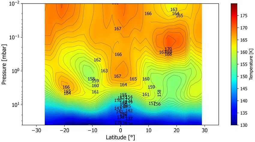
A&A 652, A125 (2021)

horizontally and vertically resolved stratospheric temperatures.
Recently, Antuñano et al. (2021) showed that Jupiter’s QQO
does not have a stable periodicity, and alterations could result
from thermal perturbations (Giles et al. 2020). Here, we there-
fore refer to the Jupiter equatorial oscillation (JEO) rather than
the QQO. We note that such perturbations have also been
seen in the SSAO following the Great Storm of 2010–2011
(Fletcher et al. 2017).
     Flasar et al. (2004) derived the JEO wind structure at low lat-
itudes from Cassini/CIRS temperature measurements performed
during the Jupiter flyby in late 2000. Invoking thermal wind
balance, these authors discovered a ∼140 m s−1 eastward equato-
rial jet at 3 mbar by interpolating wind velocities, even though
a precise estimate of the jet peak velocity at the equator is
made impossible because of the increase in the Rossby number.
Fletcher et al. (2016) confirmed the presence of a strong strato-      Fig. 1. Eastward wind velocities at 1 mbar as measured with ALMA on
spheric jet in the mbar region. Cosentino et al. (2017) were able      22 March 2017, on the eastern and western limbs of Jupiter (adapted
to reproduce such JEO wind speeds to first order using an atmo-        from Cavalié et al. 2021).
spheric circulation model with a stochastic parametrization of
gravity wave drag.
     Fouchet et al. (2008) found a velocity difference of about
200 m s−1 in Saturn’s stratosphere between the two equatorial
jets located at 0.3 and 3 mbar, also applying the thermal wind
balance to the measured temperatures. However, the absolute
stratospheric wind speeds remain unknown on Saturn (and were
unknown until now for Jupiter), and given the strong eastward
cloud-top zonal wind of 400 m s−1 observed at ∼700 mbar, it
is unsure whether the stratospheric wind remains eastward or
becomes periodically westward, as observed on Earth.
     The main weakness in the methodology used in previous
studies to derive the thermal winds, and particularly in the case
of Jupiter, is that there is a discontinuity between the pressure
range probed by the temperatures (1–20 mbar from CH4 emis-
sion, 80–400 mbar from H2 collision-induced absorption) and
the pressure at which the zonal wind profile is inserted as a          Fig. 2. Mean eastward wind velocities (green line) with uncertainties
                                                                       (green bars) at 1 mbar in Jupiter’s stratosphere on 22 March 2017. A
boundary condition, i.e., generally at the cloud-top (at 500 mbar)
                                                                       degree 35 Legendre polynomial smoothing is plotted with dashed red
during the thermal wind derivation. The novelty of the approach        lines.
we present here consists in using a wind measurement performed
almost concomitantly and within the altitude range probed by
the stratospheric temperature measurements. We are thus able to        spectral lines formed at the altitude probed by the HCN line.
obtain self-consistent zonal wind field as a function of altitude      The latitudinal resolution varies from 3◦ at the equator to 7◦ at
and latitude in the whole range probed by the temperature mea-         polar latitudes. Contribution function computations demonstrate
surements. In this paper, we focus on Jupiter’s zonal winds in the     that the sensitivity to winds peaks at 1 mbar in the 60◦ S–50◦ N
altitude and latitude ranges where the JEO takes place in order        latitudinal range, and at 0.1 mbar at polar latitudes. In this paper,
to constrain the direction and magnitude of the equatorial and         we use the data ranging from 35◦ S to 35◦ N planetocentric lat-
tropical jets using the thermal wind balance.                          itude. Although the data were acquired with a short 24-min
     In Sect. 2, we present the wind and temperature observa-          on-source integration time, the rapid rotation of the planet (9 hr
tions we used to compute the zonal wind field. Section 3 details       56 min) results in longitudinal smearing over about 15◦ . The cen-
the models we developed to compute the equatorial and trop-            tral meridian longitude thus ranges from 65◦ W to 80◦ W (System
ical wind speeds from the thermal wind balance. We present             III). The eastern and western limbs (From the observer’s point of
our results and discuss them in Sect. 4, and provide concluding        view) span longitudes from 335◦ W to 350◦ W and from 155◦ W
remarks in Sect. 5.                                                    to 170◦ W, respectively. The eastward wind velocities obtained by
                                                                       Cavalié et al. (2021) are shown for both observed limbs in Fig. 1.
                                                                       The average of both limb measurements are shown in Fig. 2.
2. Observations
2.1. Zonal wind measurements at 1 mbar in Jupiter’s                    2.2. Jupiter’s stratospheric temperature field observations
     stratosphere
                                                                       In March 2017, TEXES (Lacy et al. 2002), mounted on the Gem-
Cavalié et al. (2021) observed Jupiter’s stratospheric HCN emis-       ini North 8 m telescope, carried out high-resolution infrared
sion at 354.505 GHz with the ALMA interferometer on 22                 observations of Jupiter to characterize the temperatures in its
March 2017. These authors obtained a high spectral and spatial         stratosphere. These observations were taken as part of a long-
resolution map of Jupiter’s limb from which they achieved the          term monitoring program carried out primarily at the NASA
first direct measurement of the stratospheric winds. The wind          Infrared Telescope Facility (Cosentino et al. 2017; Giles et al.
speeds were retrieved from the wind-induced Doppler-shifted            2020). TEXES can observe at wavelengths ranging from 4.5
A125, page 2 of 9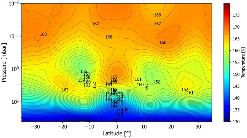
B. Benmahi et al.: Mapping the zonal winds of Jupiter’s stratospheric equatorial oscillation

                                                                           gradient with the perpendicular velocity in the (→−
                                                                                                                             eθ ; →
                                                                                                                                  −
                                                                                                                                  eφ ) plane1 of
                                                                           a fluid (such as an atmosphere) in a rotating frame. This equation
                                                                           is given by the following expression:

                                                                                        ∂→
                                                                                         −v (r, θ, φ)
                                                                                           ⊥             r → −r ∧ →
                                                                                                                  −
                                                                            f0 sin(θ)                 =           5 ⊥ T (r, θ, φ),                (1)
                                                                                             ∂r         T r0
                                                                           where f0 is the Coriolis parameter at the north pole, θ is the
                                                                           latitude varying from −90◦ to 90◦ , →  −
                                                                                                                  v⊥ (r, θ, φ) is the horizontal
                                                                           fluid velocity at the planet surface, r0 is the mean radius of the
                                                                           planet, and T is the temperature field. From this equation, and
                                                                           after projecting on the zonal axis, we can easily relate the zonal
                                                                           wind speed with the latitudinal temperature gradient. Thus, we
                                                                           have the following expression:
Fig. 3. Average of the temperature fields at the eastern and western
limbs covered by the ALMA wind observations. This temperature field          ∂vφ     1 R(P) ∂T
is referred to as the east–west limb mean in this paper and results from          =                ,                                              (2)
the average of the fields are shown in Figs. A.3 and A.4. Latitudes are    ∂ ln(P) sin(θ) f0 r0 ∂θ
planetocentric.
                                                                           where P is the pressure and vφ is the zonal wind velocity.
                                                                           R(P) = M(P)
                                                                                    kB
                                                                                        is the specific gas constant of the Jovian atmosphere
to 25 µm, with a spectral resolving power ranging from 4000                calculated for each altitude. M(P) is the mean molecular mass
to 80 000 depending on the operating mode. The observations                of Jupiter’s atmosphere as a function of pressure. We derive
of Jupiter were centered around 8.02 µm with a bandwidth of                it from the model used in Benmahi et al. (2020). Establishing
about 0.06 µm where several spectral lines of the CH4 (ν4 band)            this equation assumes hydrostatic and geostrophic equilibrium,
P-branch lie (Brown et al. 2003). During the March 2017 observ-            and the latter is guaranteed by the small Rossby number (Ro)
ing campaign, TEXES was used in its highest spectral resolution            in Jupiter’s atmosphere. As the Coriolis force vanishes at the
mode (R = 80 000).                                                         equator because of the f0 sin(θ) factor, this equation diverges at
     The Gemini/TEXES observations were used to retrieve ver-              the equator (θ = 0). This is why Flasar et al. (2004) only used
tically resolved latitude and longitude temperature maps of                the TWE down to latitudes of about 5◦ in their zonal wind
Jupiter’s stratosphere. These maps were compared to the lower              derivation.
spatial resolution maps from the IRTF to show that IRTF/TEXES
is capable of fully resolving the meridional structure of the
                                                                           3.2. Equatorial thermal wind equation
JEO (Cosentino et al. 2020). The pressure range probed by the
TEXES data ranges from 0.1 to 30 mbar with a vertical reso-                Marcus et al. (2019) derived an equatorial thermal wind equation
lution of approximately one scale height. Beyond this pressure             (EQTWE). This uses the Laplacian in latitude of the tempera-
range, the temperature vertical profiles converge toward the pro-                                     1
                                                                           tures, which allows the sin(θ) factor of the TWE to be canceled
file from Moses et al. (2005), which is taken as a priori for the          out. As a result, the EQTWE does not diverge at low latitudes
retrievals. The horizontal resolution is 2◦ in latitude and 4◦ lon-        and is thus particularly useful for replacing the TWE in the
gitude. The uncertainty on the retrieved temperatures is about             equatorial zone. Its expression is given by:
2 K.
     The Gemini/TEXES temperature field we use in this paper                   ∂vφM       R(P) ∂2 T M
was retrieved from the combined data taken on 14, 16, and 20                          =               ,                                           (3)
March 2017, i.e., only 2–8 days apart from the ALMA wind mea-              ∂ ln(P)        f0 r0 ∂θ2
surements. By extracting the temperatures at the longitudes of
the limbs probed by ALMA and accounting for the 15◦ longitu-               where T M (P, θ) = T (P,θ)+T     2
                                                                                                              (P,−θ)
                                                                                                                     is the mirror-symmetric
dinal smearing, we produced altitude–latitude temperature fields           component of the temperature about the equator. The
for each limb, and an average of both. The latter, referred to as          anti-mirror-symmetric component of the temperature is
the east–west limb mean in what follows, is shown in Fig. 3.               T A (P, θ) = T (P,θ)−T
                                                                                                2
                                                                                                  (P,−θ)
                                                                                                         . According to Marcus et al. (2019), the
                                                                                                                         A
The former are shown in Figs. A.3 and A.4, and the zonal mean              EQTWE has a fractional error of ∝ | TT M |2 , and is valid in the
temperature field is shown in Fig. A.1 for comparison. We note,                                           ◦
                                                                           latitudinal range +/−18 with an error of less than 10%.
however, that we only have full longitudinal coverage over the                  The derivation of the EQTWE requires the same assump-
eastern limb. Only one-third of the western limb (155◦ –170◦ W)            tions as for the TWE, except the limitations regarding the Rossby
is covered by temperature measurements (155◦ –160◦ W).                     number at the equator, and assumes that the flow is symmetrical
                                                                           around the equator (see Appendix A in Marcus et al. 2019).

3. Models                                                                  3.3. Assumptions and equation solving
3.1. Thermal wind equation                                                 To carry out our study, we must also assume that Jupiter’s
                                                                           temperature field remains stationary over the time interval
Atmospheric dynamics can be interpreted with the equations of              between the TEXES thermal and ALMA wind measurements
fluid mechanics. The so-called thermal wind equation (TWE)                 (from 2 to 8 days). This is justified for several reasons: The
derives from Euler’s equations for a frictionless fluid (e.g.,
Pedlosky 1979). In spherical coordinates and assuming                      1 The unit vector → −
                                                                                               eφ is oriented in the direction of the planet rotation
geostrophic equilibrium, the TWE relates the temperature                   such that positive winds are eastward.

                                                                                                                                     A125, page 3 of 9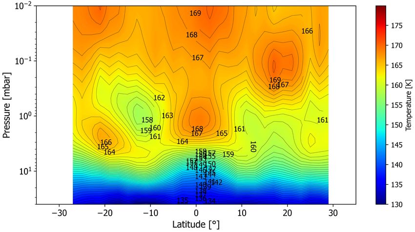
A&A 652, A125 (2021)
characteristic time of variability of cloud and storm dynamics
in the troposphere is about a few days. However, their effects on
stratospheric temperatures are transported by wave and energy
propagation on timescales comparable to the periodicity of the
JEO. Moreover, seasonal effects on Jupiter are weak (e.g., Hue
et al. 2018) and the considered duration is negligible compared
to Jupiter’s year, and is considered to be much shorter than
the radiative timescales in Jupiter’s stratosphere (Guerlet et al.
2020).
Before solving the TWE and EQTWE, we smoothed the tem-
perature field and the 1-mbar wind speeds over latitude in order
to obtain smooth and continuous derivatives (see Appendix C).
We smoothed the various temperature fields (the east–west limb
Fig. 4. Examples of Legendre polynomial series fitting of the temper-
mean of Fig. 3, the zonal average of Fig. A.1, the eastern and
atures as a function of latitude for four different pressure levels. The
western limbs of Figs. A.3 and A.4) with a Legendre polynomial two lower pressure profiles (0.1 and 1.1 mbar) are from the Giles et al.
series up to degree 17. An example of fits at several pressures (2020) dataset that we primarily use in this paper. The higher pressure
is shown in Fig. 4. For the ALMA wind velocities at 1 mbar, we profiles (39.8 and 98 mbar) are from the Fletcher et al. (2020) dataset.
used a Legendre polynomial series up to degree 35 (see Fig. C.1). Fits are in solid lines and data are shown with symbols and error bars of
We determined the highest degree of the fitting polynomials such corresponding color.
that the fits were within observation uncertainties. For tempera-
tures and velocities, we used a latitudinal sampling of 0.25◦ and
we solved the TWE and EQTWE with this sampling from 35◦ S
to 35◦ N. We integrated the equations upwards and downwards
starting with the ALMA wind velocities as initial conditions at
P0 = 1 mbar.
Finally, we need to determine the latitude range around the
equator in which we solve the EQTWE and then switch to the
TWE. The TWE is highly dependent on Ro and its fractional
error is about ∝ Ro. We therefore estimate Ro as a function of lat-
itude by considering a characteristic velocity scale for Jupiter’s
atmosphere of 100 m s−1 . We find Ro ∼ 0.2 at +/−5◦ latitude.
We therefore solve the EQTWE on the mirror-symmetric com-
ponent of the temperature field T M (P, θ) in the latitude interval
[−3◦ ; 3◦ ], where the initial velocity condition vφ (θ, P0 ) (i.e., the
fitted curve in Fig. 2) is actually quasi-symmetrical about the
equator. We then solve the TWE in the latitude interval [−35◦ ;
−5◦ ] ∪ [5◦ ; 35◦ ] using T (P, θ). Finally, we use a bilinear interpo-
lation between the two results in the [−5◦ ; −3◦ ] ∪ [3◦ ; 5◦ ] range
to combine the results into a single map.
4. Results and discussion
4.1. Zonal winds in the JEO region
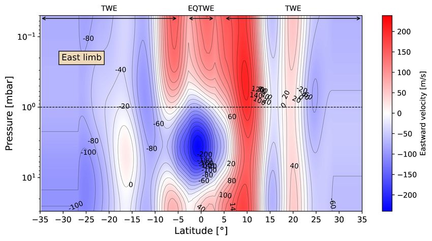
Figure 5 (top) shows the eastward wind velocities that we derive
from the east–west limb mean temperature map of Fig. 3 with the
EQTWE and TWE and using the wind speeds measured with
ALMA at 1 mbar (Fig. 2) as an initial condition. We note that Fig. 5. Top: eastward wind velocities derived from the east–west limb
there is no sharp discontinuity between the two equation solu- mean temperature map of Fig. 2 and the measured winds at 1 mbar of
tions in the [−5◦ ; −3◦ ] ∪ [+3◦ ; +5◦ ] latitude range and from 0.5 Fig. 3 with the EQTWE and TWE. The dashed horizontal line repre-
to 30 mbar. Above the 0.5 mbar pressure level in the united lat- sents the altitude where stratospheric winds were measured by Cavalié
itude range [−5◦ ; −3◦ ] ∪ [3◦ ; 5◦ ], we notice small differences et al. (2021). Bottom: wind shear as obtained from the east–west limb
mean temperature field.
between the two equation solutions. Because the TWE is highly
dependent on the Rossby number, its validity also depends on it.
Thus, the discrepancy between the TWE and the EQTWE is due (two scale heights). At pressures lower than 1 mbar, we find an
to the local variability of the Rossby number. eastward jet, which is 20◦ wide in latitude and has a FWHM of
We present these computations in the 0.05–30 mbar range about 80 km in altitude (between 0.05 and 0.5 mbar). The vertical
(e.g., Fig. 5), where the TEXES observations are sensitive to stratification about the equator is also unambiguously character-
temperatures and have the lowest uncertainties in the retrievals. ized, with a peak-to-peak difference of 300 m s−1 between 4 mbar
The JEO can clearly be identified in the zonal wind map by ver- and 0.1 mbar. The JEO jet in March 2017 is almost perfectly in
tically alternating zonal jets. We find a strong westward (i.e., opposition of phase compared to the state observed by Flasar
retrograde) jet at the equator centered at about 4 mbar with a et al. (2004) in December 2000 at the time of the Cassini flyby.
peak velocity of 200 m s−1 . This jet has a full-width at half- The amplitudes of the JEO jet in these two observations are com-
maximum (FWHM) of about 7◦ in latitude and 50 km in altitude parable (200 m s−1 vs. 140 m s−1 ), even though the exact velocity
A125, page 4 of 9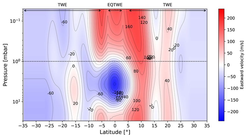
B. Benmahi et al.: Mapping the zonal winds of Jupiter’s stratospheric equatorial oscillation

at the equator is not known in Flasar et al. (2004) because of
the limitations of the TWE at the equator. At ∼10◦ N, the east-
ward jet is vertically extended over the entire pressure range with
an average velocity of 125 m s−1 . Beyond +/−15◦ , winds have
amplitudes lower than 40 m s−1 .
                                                    ∂v
    In Fig. 5 (bottom), we map the wind shear ( ∂rφ ) as obtained
from the east–west limb mean temperature field (Fig. 3). We can
clearly see two wind shear spots centered around the equator,
with positive and negative amplitudes of ∼160 m s−1 /H above
and below the ∼4 mbar pressure level, respectively, where the
westward jet is located (Fig. 5). The two wind shear spots have
a FWHM of about 12◦ in latitude. Beyond +/−10◦ latitude, the
wind shear is negligible. Such vertical and latitudinal extensions
and amplitudes are comparable to previous estimates (Fletcher
et al. 2016; Marcus et al. 2019).
    The zonal wind map we obtained from the Gemini/TEXES
measurements in March 2017 combined with the 1 mbar zonal
wind measured by Cavalié et al. (2021) using ALMA and the
result obtained by Fletcher et al. (2016) from the zonal temper-
ature field measured by IRTF/TEXES in December 2014 are of
almost opposite phase in the 1–10 mbar range. The time-interval
between the two measurements is ∆T ∼2 yr and 4 months. This
would lead to a JEO period of 4 yr and 8 months, in agree-
ment with previous measurements (Leovy et al. 1991; Orton et al.
1991). We note that Antuñano et al. (2021) has now demonstrated
that this periodicity is variable and can even be disrupted, as
observed by Giles et al. (2020). Such disruptions may originate
from the outbreak of thermal anomalies like the one seen in May          Fig. 6. Eastward zonal wind velocities mapped independently at the
2017 at 1 mbar pressure, 20◦ N latitude, and 180◦ W longitude            western (top) and the eastern (bottom) limbs.
(See Fig. 7 in Giles et al. 2020).
                                                                         data. Eastward–westward wind velocities at the northern and
4.2. Longitudinal variability of zonal winds in the JEO region           southern boundaries of an anticyclonic feature can reach 100–
                                                                         150 m s−1 , as in the Great Red Spot (Choi et al. 2007). In the
The wind velocity maps we derive from the temperature zonal              stratosphere, the most famous example of an anticyclonic fea-
mean, from the eastern limb only, and from the western limb only         ture was observed in Great Storm on Saturn in 2010–2011. At
(Figs. A.1, A.3, and A.4, respectively) are presented in Figs. A.2,      2 mbar, Fletcher et al. (2012) estimated zonal wind velocities
and 6, respectively. The two latter wind maps are obtained using         at the northern and southern boundaries of the vortex in the
the eastern and western ALMA wind measurements of Fig. 1 as              200–400 m s−1 range. Therefore, the 100 m s−1 lower velocity
initial condition.                                                       observed on the 10◦ N jet on the western limb in the ALMA data
     We notice in Fig. 6 that the 10◦ N wind peak observed at            (compared to the eastern limb) could be at least partly explained
1 mbar with ALMA can be tracked down to the lower strato-                by the presence of an anticyclonic feature centered at 15◦ N.
sphere, where it is centered around 7◦ N. This latitude is where             The winds obtained from the east–west limb mean (Fig. 5)
the northern peak of the double-horned structure is observed             and those obtained from the zonal mean (Fig. A.2) are very sim-
around the equator at the cloud-top (Barrado-Izagirre et al.             ilar in the +/−10◦ latitude range, indicating that the east–west
2013). The eastward jet at 10◦ N and 1 mbar and the one at 7◦ N          limb mean in both winds and temperatures at 1 mbar was a fair
and 30 mbar seem to be linked. Indeed, the eastward column con-          representation of the zonal mean on this occasion. The westward
necting the two altitudes (1 and 30 mbar) seems to be distorted by       equatorial jet at 4 mbar has a similar shape and amplitude. Out-
the central westward jet at 4 mbar. We think that these two peaks        side this range, the differences are less than 20 m s−1 , which is
are correlated and connected vertically, and that the presence           about the HCN wind measurement uncertainty with ALMA.
of the westward jet, and thus of the planetary wave generating               More significant differences arise when we compare the
the JEO, results in a latitudinal shift between the two eastward         winds obtained from the two limb temperatures independently
peaks at 1 mbar and at 30 mbar. The peak at 7◦ N and 30 mbar is          (Fig. 6). The westward equatorial jet at 4 mbar is 50 m s−1
likely tied to the cloud-top northern branch of the double-horned        stronger on the eastern limb than on the western limb. On the
structure mentioned above.                                               eastern limb, we also notice that the northern equatorial branch
     A subject of debate in Cavalié et al. (2021) was the limb-to-       centered around 7◦ –10◦ N of the upper stratospheric eastward jet
limb velocity difference at 10◦ N, which the authors tentatively         is 50–75 m s−1 stronger than in the western limb. Both extend
attributed to local vortices. The lack of full coverage of the           down to the lower boundary of our calculations (30 mbar). The
western limb temperatures prevents us from settling this claim,          distinct eastward barotropic jet at 20◦ N disappears on the western
although the limited data we have seem to indicate the pres-             limb.
ence of a hot spot between 10◦ N and 15◦ N and between 1                     By comparing the 4 mbar equatorial westward jet velocities
and 2 mbar as seen in Fig. B.1. This hot spot, if anticyclonic,          in the two limbs (Fig. 6), we find a difference of about 50 m s−1 .
would decelerate the winds about ∼10◦ N and accelerate the               This results from a combination of the differences between the
wind about ∼20◦ N, in qualitative agreement with the ALMA                velocities measured at 1 mbar and the temperatures in the two
                                                                                                                           A125, page 5 of 9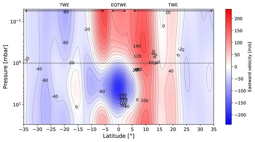
A&A 652, A125 (2021)

Fig. 7. Temperature field resulting from the combination of retrievals
obtained from the high-spectral-resolution observations of Cosentino
et al. (2020) (Fig. 3) and the retrievals from the lower spectral resolution
observations of Fletcher et al. (2020), all performed between 12 and 20
March, 2017. This temperature field covers the 0.05–1000 mbar pressure
range.

                                                                               Fig. 9. Vertical profile of the temperature at the equator extracted from
                                                                               the field of Fig. 7 from the combination of retrievals obtained from the
                                                                               high-spectral-resolution observations of Giles et al. (2020) (Fig. 3) and
                                                                               the retrievals from the lower spectral resolution observations of Fletcher
                                                                               et al. (2020), all performed between 12 and 20 March 2017. The two
                                                                               profiles are averaged in the 20–30 mbar pressure range (referred to as
                                                                               the overlapping zone on the plot).

Fig. 8. Comparison between the cloud-top wind speeds measured at
500 mbar in the visible (red points with error bars) with the thermal
winds (dashed magenta line) derived from the east–west mean temper-                In Fig. 8, we compare the zonal wind profile calculated at
ature field of Fig. 3 and the 1mbar wind observations with ALMA of             500 mbar with the cloud-top wind observations performed in
Fig. 2 (blue solid line).                                                      the visible range (e.g., Barrado-Izagirre et al. 2013). Our ther-
                                                                               mal wind results at 500 mbar show a strong wind speed increase
                                                                               within ±10◦ , as expected from observations. However, we do not
limbs. The differences we find in the equatorial temperatures                  reproduce the double-horned shaped centered about the equator.
between the two limbs and between 1 and 4 mbar are twice the                   Instead, we see that the TWE and EQTWE do not provide con-
longitudinal standard deviation in this pressure range.                        sistent results in the [−5◦ ; −3◦ ] ∪ [3◦ ; 5◦ ] ranges because of the
                                                                               longer vertical integration that causes larger deviations between
                                                                               the two solutions. In addition, the wind speeds around the equa-
4.3. Equatorial cloud-top wind structure                                       tor are overestimated by a factor of approximately two within
                                                                               ±10◦ . This deviation probably arises from the different vertical
We checked whether the temperature and wind observations                       resolutions in the two temperature retrievals that we combined to
combined with our model allow derivation of the cloud-top wind                 perform these computations. The lower vertical resolution of the
structure. To this end, we extended our east–west limb mean tem-               upper tropospheric–lower stratospheric temperatures is in turn
perature map (Fig. 3) down to upper tropospheric altitudes. To                 caused by the lower spectral resolution of the observations of
do so, we used the upper tropospheric and lower stratospheric                  Fletcher et al. (2020) compared to those of Giles et al. (2020).
temperatures as retrieved by Fletcher et al. (2020) from lower                 In addition, the deviation may also result from the higher uncer-
spectral resolution Gemini/TEXES observations taken on 12–14                   tainties in the temperatures retrieved by Fletcher et al. (2020)
March 2017 and probed in the pressure range p < 1000 mbar. We                  (on average ±4 K compared to the ±2 K of Giles et al. 2020).
combined the two temperature fields by averaging them between                  These higher uncertainties in the higher pressures can be better
20 and 30 mbar for the relevant longitudes. This pressure range is             seen in Fig. 9, where we present a vertical temperature profile
chosen so as to minimize the overlap and thus favor the temper-                at the equator resulting from the combination of the tempera-
atures retrieved from the high-spectral-resolution observations                ture fields of Giles et al. (2020) and Fletcher et al. (2020). These
at least down to the pressure level of 20 mbar. The resulting                  higher uncertainties in the higher pressures can also been seen
thermal map is shown in Fig. 7 and covers pressures from 0.05                  in Fig. 4. We finally tried to integrate the temperature field start-
to 1000 mbar. We then applied our thermal wind model, still                    ing from the cloud-top wind speeds. The wind speeds we obtain
using the ALMA wind measurements as the initial condition at                   at 1 mbar (not shown here) are in total disagreement with the
1 mbar.                                                                        ALMA observations.
A125, page 6 of 9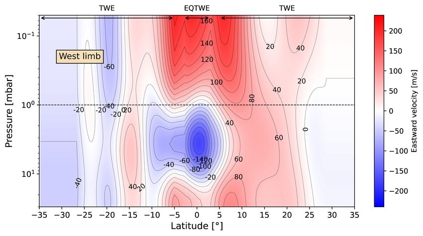
B. Benmahi et al.: Mapping the zonal winds of Jupiter’s stratospheric equatorial oscillation

5. Conclusion                                                            Explorer. The technique presented in this paper can certainly
                                                                         be adapted to the other giant planets to study their general
The main outcomes of this paper can be summarized as follow:             circulation and equatorial oscillations.
  – We used the recent and first measurements of the Jovian
    stratospheric winds obtained from ALMA observations                  Acknowledgements. This work was supported by the Programme National de
    (Cavalié et al. 2021), with the temperature field obtained           Planétologie (PNP) of CNRS/INSU and by CNES. The authors thank L. N.
    almost simultaneously in March 2017 in the mid-infrared              Fletcher for providing them with the temperature retrievals of his 2016 paper.
                                                                         Coauthors Guerlet and Spiga acknowledge funding from Agence Nationale de la
    from Gemini/TEXES observations (Giles et al. 2020), to               Recherche (ANR) project EMERGIANT ANR-17-CE31-0007.
    derive the zonal wind field as a function of pressure and lat-
    itude in the equatorial zone of Jupiter’s stratosphere where
    the Jupiter equatorial oscillation occurs.                           References
  – We used the thermal wind equation, complemented by the
                                                                         Antuñano, A., Cosentino, R. G., Fletcher, L. N., et al. 2021, Nat. Astron., 5, 71
    equatorial thermal wind equation of Marcus et al. (2019) for         Baldwin, M. P., Gray, L. J., Dunkerton, T. J., et al. 2001, Rev. Geophys., 39, 179
    the latitudes about the equator, to derive the Jovian strato-        Bardet, D., Spiga, A., Guerlet, S., et al. 2021, Icarus, 354, 114042
    spheric zonal winds from 0.05 to 30 mbar and from 35◦ S to           Barrado-Izagirre, N., Rojas, J. F., Hueso, R., et al. 2013, A&A, 554, A74
    35◦ N.                                                               Benmahi, B., Cavalié, T., Dobrijevic, M., et al. 2020, A&A, 641, A140
                                                                         Brown, L. R., Benner, D. C., Champion, J. P., et al. 2003, J. Quant. Spectr. Rad.
  – We derive the absolute stratospheric zonal wind speeds ±35◦             Transf., 82, 219
    about the equator, where the JEO takes place. We thus pro-           Cavalié, T., Benmahi, B., Hue, V., et al. 2021, A&A, 647, L8
    vide the general circulation modeling community with the             Choi, D. S., Banfield, D., Gierasch, P., & Showman, A. P. 2007, Icarus, 188, 35
    first full diagnostic of the JEO zonal winds for a given date.       Cosentino, R. G., Morales-Juberías, R., Greathouse, T., et al. 2017, J. Geo-
  – In March 2017, we find a strong westward (i.e., retrograde)             phys. Res., 122, 2719
                                                                         Cosentino, R. G., Greathouse, T., Simon, A., et al. 2020, Planet. Sci. J., 1, 63
    jet centered on the equator and about the 4 mbar level with a        Ebdon, R. A., & Veryard, R. G. 1961, Nature, 189, 791
    peak velocity of 200 m s−1 . The vertical stratification of the      Flasar, F. M., Kunde, V. G., Achterberg, R. K., et al. 2004, Nature, 427, 132
    JEO winds is demonstrated and we find that the westward jet          Fletcher, L. N., Hesman, B. E., Achterberg, R. K., et al. 2012, Icarus, 221, 560
    lies beneath a broader eastward (i.e., prograde) jet and the         Fletcher, L. N., Greathouse, T. K., Orton, G. S., et al. 2016, Icarus, 278, 128
                                                                         Fletcher, L. N., Guerlet, S., Orton, G. S., et al. 2017, Nat. Astron., 1, 765
    peak-to-peak contrast is ∼300 m s−1 .                                Fletcher, L. N., Orton, G. S., Greathouse, T. K., et al. 2020, J. Geophys. Res.,
  – We find longitudinal variability at the level of ∼50 m s−1              125, 8
    when comparing the winds derived independently from the              Fouchet, T., Guerlet, S., Strobel, D. F., et al. 2008, Nature, 453, 200
    eastern and western limbs of the ALMA observations, even             Friedson, A. J. 1999, Icarus, 137, 34
    though the overall structure of the JEO remains similar.             Giles, R. S., Greathouse, T. K., Cosentino, R. G., Orton, G. S., & Lacy, J. H.
                                                                            2020, Icarus, 350, 113905
  – When extending our zonal wind computations to the cloud-             Guerlet, S., Fouchet, T., Bézard, B., Flasar, F. M., & Simon-Miller, A. A. 2011,
    top using complementary thermal data (also taken over the               Geophys. Res. Lett., 38, L09201
    same time period), we tentatively find a global wind structure       Guerlet, S., Fouchet, T., Spiga, A., et al. 2018, J. Geophys. Res., 123, 246
    close to observations. We find a strong equator-centered pro-        Guerlet, S., Spiga, A., Delattre, H., & Fouchet, T. 2020, Icarus, 351, 113935
                                                                         Hue, V., Hersant, F., Cavalié, T., Dobrijevic, M., & Sinclair, J. A. 2018, Icarus,
    grade jet. However, the lower spectral resolution of the lower          307, 106
    stratospheric and upper tropospheric temperature observa-            Lacy, J., Richter, M., Greathouse, T., Jaffe, D., & Zhu, Q. 2002, PASP, 114,
    tions prevent a closer and more quantitative agreement. We              153
    recover neither the double-horned equatorial shape nor the           Leovy, C. B., Friedson, A. J., & Orton, G. S. 1991, Nature, 354, 380
    20◦ N jet.                                                           Li, X., & Read, P. L. 2000, Planet. Space Sci., 48, 637
                                                                         Lindzen, R. S., & Holton, J. R. 1968, J. Atmos. Sci., 25, 1095
Such direct stratospheric wind and temperature measurements,             Marcus, P. S., Tollefson, J., Wong, M. H., & Pater, I. d. 2019, Icarus, 324, 198
performed almost simultaneously, provide a new and promis-               Moses, J. I., Fouchet, T., Bézard, B., et al. 2005, J. Geophys. Res., 110, E08001
ing way to characterize and understand the Jupiter equatorial            Orton, G. S., Friedson, A. J., Caldwell, J., et al. 1991, Science, 252, 537
oscillation and, more globally, its general circulation. Repeated        Orton, G. S., Yanamandra-Fisher, P. A., Fisher, B. M., et al. 2008, Nature, 453,
                                                                            196
observations on various timescales are now needed to accom-              Pedlosky, J. 1979, Geophysical Fluid Dynamics (New York: Springer-Verlag)
plish this goal. These can be achieved first with ALMA and               Reed, R. J., Campbell, W. J., Rasmussen, L. A., & Rogers, D. G. 1961,
ground-based infrared facilities, and later on with the Sub-                J. Geophys. Res., 66, 813
millimetre Wave Instrument on board the Jupiter Icy Moons                Simon-Miller, A. A., Conrath, B. J., Gierasch, P. J., et al. 2006, Icarus, 180, 98

                                                                                                                                      A125, page 7 of 9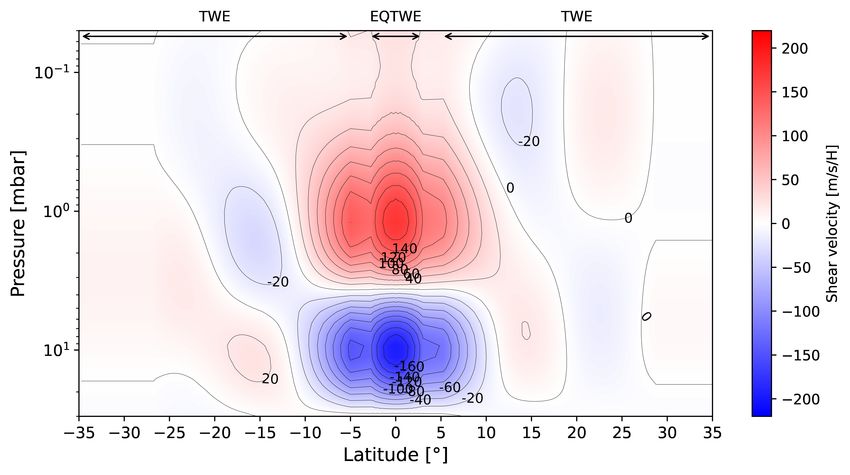
A&A 652, A125 (2021)

Appendix A:
Thermal wind velocities from alternative
temperature maps
Figure A.1 presents the zonal mean of the temperatures in
Jupiter’s stratosphere from 0.01 to 30 mbar on 12-20 March
2017. The corresponding wind velocity map is shown in
Figure A.2.

                                                                         Fig. A.3. Eastern limb temperature field resulting from the average
                                                                         between 335◦ and 350◦ longitudes, as observed with Gemini/TEXES
                                                                         on 14, 16, and 20 March 2017.

Fig. A.1. Zonal mean of the Jovian stratospheric temperature field, as
observed with Gemini/TEXES on 14, 16, and 20 March, 2017.

                                                                         Fig. A.4. Western limb temperature field resulting from the average
                                                                         between 155◦ and 160◦ longitudes, as observed with Gemini/TEXES
                                                                         on 14, 16, and 20 March 2017. There is no data between 160◦ and 170◦ ,
                                                                         preventing thus a full coverage of this limb.

                                                                         This hot spot may partly explain the differences in wind speeds
                                                                         notably observed around 10◦ N in the two limbs with ALMA
                                                                         (Figure 1). Anticyclonic motions about this spot would decrease
Fig. A.2. Eastward zonal wind velocities derived from the zonal mean     the wind speeds at 10◦ N, and increase the wind speeds at 20◦ N
temperature field of Figure A.1 and from the 1 mbar winds of Figure 2.   on the western limb with respect to the zonal average. On the
                                                                         contrary, the eastern limb shows a cold spot at 2 mbar and cen-
    We also produced the temperature maps from the Gem-                  tered at 22◦ N. Here, cyclonic motions about this cold spot would
ini/TEXES data for the two longitude ranges covered by the               tend to increase wind speeds at ∼17◦ N, and decrease them at
limbs observed with ALMA, after accounting for the 15◦ longi-            ∼26◦ N on the eastern limb with respect to the zonal average. This
tudinal smearing of these observations. These temperature maps           would qualitatively tend to bring the wind speed profiles from the
are shown in Figures A.3 and A.4. The corresponding wind                 two limbs of Figure 1 back into agreement, mostly regarding the
velocity maps are presented in Figure 6.                                 differences seen on the 10◦ N prograde jet.

Appendix B:                                                              Appendix C:
Longitudinal variability of the temperatures in                          Wind and temperature data smoothing method
March 2017
                                                                         Before using the wind speeds and temperatures that come from
We computed the difference between the Gemini/TEXES tem-                 the observations in our modeling, we smoothed the data with
peratures averaged over the western limb and the zonal mean,             Legendre polynomial series. We first determined the order of the
and proceeded similarly for the eastern limb. The results are            highest order n of the series to smooth our data, such that the
shown in Figures B.1 and B.2.                                            fit lies within all uncertainties. For the wind speeds of Figure 2,
    We find that the western limb presents a hot spot centered at        we set n = 35. For the temperature as a function of latitude (and
15◦ N and extended over 10-15◦ in latitude between 1 and 2 mbar.         for each altitude), we set n = 17. Such polynomials can result in
A125, page 8 of 9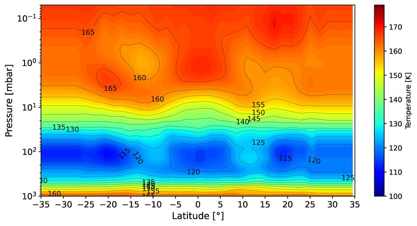
B. Benmahi et al.: Mapping the zonal winds of Jupiter’s stratospheric equatorial oscillation

Fig. B.1. Difference between western limb temperatures and the zonal
mean.

Fig. B.2. Difference between eastern limb temperatures and the zonal
mean.

edge effects like the Gibbs phenomenon. To avoid this effect, we
had to extrapolate the velocity and temperature curves beyond
the latitude range we used in our modeling (i.e., from -35◦ to
+35◦ ). We extended the latitudinal range up to +/-50◦ and applied
the fit. The results regarding the wind speeds can be found in
Figure C.1, where the Gibbs-like effect can be seen around +/-
50◦ . This effect is thus avoided in the final latitude range we use
in our work.

Fig. C.1. Legendre polynomial series smoothing of the ALMA wind
speeds. We extend the fitting range from ±35◦ to ±50◦ to limit the edge
effects of such a fitting procedure to outside the studied interval. The
resulting fit is then truncated to the interval of interest.

                                                                                                                           A125, page 9 of 9
You can also read