Phillies Tweeting from Philly? Predicting Twitter
←
→
Page content transcription
If your browser does not render page correctly, please read the page content below
@Phillies Tweeting from Philly? Predicting Twitter
     User Locations with Spatial Word Usage
                      Hau-Wen Chang∗ , Dongwon Lee∗ , Mohammed Eltaher† and Jeongkyu Lee†
                             ∗   The Pennsylvania State University, University Park, PA 16802, USA
                                              Email: {hauwen|dongwon}@psu.edu
                                     † University of Bridgeport, Bridgeport, CT 06604, USA

                                         Email: {meltaher|jelee}@bridgeport.edu

   Abstract—We study the problem of predicting home locations        to hang out, cheer a player in local sports team, or discuss
of Twitter users using contents of their tweet messages. Using       local candidates in elections. Therefore, it is natural to take
three probability models for locations, we compare both the          this observation into consideration for location estimation.
Gaussian Mixture Model (GMM) and the Maximum Likelihood
Estimation (MLE). In addition, we propose two novel unsu-            A. Related Work
pervised methods based on the notions of Non-Localness and
Geometric-Localness to prune noisy data from tweet messages.            The location estimation problem which is also known as
In the experiments, our unsupervised approach improves the           geolocating or georeferencing has gained much interests re-
baselines significantly and shows comparable results with the        cently. While our focus in this paper is on using “textual” data
supervised state-of-the-art method. For 5,113 Twitter users in the   in Twitter, a similar task using multimedia data such as photos
test set, on average, our approach with only 250 selected local
                                                                     or videos (along with associated tags, description, images
words or less is able to predict their home locations (within 100
miles) with the accuracy of 0.499, or has 509.3 miles of average     features, or audio features) has been explored (e.g., [11], [12],
error distance at best.                                              [6], [8]). Hecht et al [5] analyzed the user location filed in user
                                                                     profile and used Multinomial Naive Bayes to estimate user’s
                      I. I NTRODUCTION                               location in state and country level.
   Knowing users’ home locations in social network systems              Current state-of-the-art approach, directly related to ours, is
bears an importance in applications such as location-based           by [3] that use a probabilistic framework to estimate city-level
marketing and personalization. In many social network sites,         location based on the contents of tweets without considering
users can specify their home locations along with other demo-        other geospatial clues. Their approach achieved the accuracy
graphics information. However, often, users either do not pro-       on estimating user locations within 100 miles of error margin,
vide such geographic information (for laziness or privacy con-       (at best) varying from 0.101 (baseline) to 0.498 (with local
cern) or provide them only in inconsistent granularities (e.g.,      word filtering). While their result is promising, their approach
country, state, or city) and reliabilities. Therefore, recently,     requires a manual selection of local words for training a
being able to automatically uncover users’ home locations            classification model, which is neither practical nor reliable.
using their social media data becomes an important problem.          A similar study proposed by [2] took a step further by taking
In general, finding the geographic location of a user from the       the “reply-tweet” relation into consideration in addition to the
user-generated contents (that are often a mass of seemingly          text contents. [7] approached the problem with a language
pointless conversations or utterances) is challenging. In this       model with varying levels of granularities, from zip codes to
paper, we focus on the case of Twitter users and try to              country levels. [4] studied the problem of matching a tweet
predict their city locations based on only the contents of their     to an object from a list of objects of a given domain (e.g.,
tweet messages, without using other information such as user         restaurants) whose geolocation is known. Their study assumes
profile metadata or network features. When such additional           that the probability of a user tweeting about an object depends
information is available, we believe one can estimate user           on the distance between the user’s and the object’s locations.
locations with a better accuracy and will leave it as a future       The matching of tweets in turn can help decide the user’s
work. Our problem is formalized as follows:                          location. [9] studied the problem of associating a single tweet
                                                                     to a tag of point of interests, e.g., club, or park, instead of
Problem 1 For a user u, given a set of his/her tweet messages        user’s home location.
Tu = {t1 , ..., t|Tu | }, where ti is a tweet message up to 140
                                                                     Our contributions in this paper are as follows: (1) We provide
characters, and a list of candidate cities, C, predict a city c (∈
                                                                     an alternative estimation via Gaussian Mixture Model (GMM)
C) that is most likely to be the home location of u.
                                                                     to address the problems in Maximum Likelihood Estimation
   Intuition behind the problem is that geography plays an           (MLE); (2) We propose unsupervised measures to evaluate the
important role in our daily lives so that word usage patterns        usefulness of tweet words for location prediction task; (3) We
in Twitter may exhibit some geographical clues. For example,         compared 3 different models experimentally with proposed
users often tweet about a local shopping mall where they plan        GMM based estimation and local word selection methods;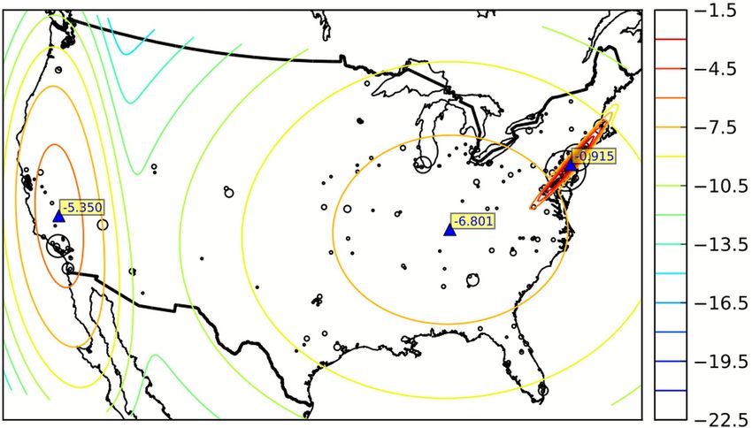
and (4) We show that our approach can, using only less than             The Maximum Likelihood Estimation (MLE) is a common
250 local words (selected by unsupervised methods), achieve a        way to estimate P (w|C) and P (C|w). However, it suffers
comparable performance to the state-of-the-art that uses 3,183       from the data sparseness problem that underestimates the
local words (selected by the supervised classification based on      probabilities of words of low or zero frequency. Various
11,004 hand-labeled ground truth).                                   smoothing techniques such as Dirichlet and Absolute Discount
                                                                     [13] are proposed. In general, they distribute the probabilities
   II. M ODELING L OCATIONS OF T WITTER M ESSAGES                    of words of nonzero frequency to the words of zero frequency.
   Recently, the generative methods (e.g., [11], [7], [12]) have     For estimating P (C|w), the probability of tweeting a word in
been proposed to solve the proposed Problem 1. Assuming              locations where there are zero or few twitter users are likely
that each tweet and each word in a tweet is generated indepen-       to be underestimated as well. In addition to these smoothing
dently, the prediction of home city of user u given his or her       techniques, some probability of a location can be distributed
tweet messages is made by the conditional probability under          to its neighboring locations, assuming that two neighboring
Bayes’s rule and further approximated by ignoring P (Tu ) that       locations tend to have similar word usages. While reported
does not affect the final ranking as follows:                        effective in other IR applications, however, the improvements
                             P (Tu |C)P (C)                          from such smoothing methods to estimate user locations have
          P (C|Tu )     =                                            been shown to be limited in the previous studies [11], [3].
                                 P (Tu )
                                    Y Y                              One of our goals in this paper is therefore to propose a
                        ∝    P (C)          P (wi |C)                better estimation for P (C|w) to improve the prediction while
                                      tj ∈Tu wi ∈tj                  addressing the spareness problem.
where wi is a word is a tweet tj . If P (C) is estimated with the
                                                                        III. E STIMATION WITH G AUSSIAN M IXTURE M ODEL
maximum likelihood, the cities having a high usage of tweets
are likely to be favored. Another way is to assume a uniform            The Backstrom model [1] demonstrated that users in a
prior distribution among cities, also known as the language          particular location tend to query some search keywords more
model approach in IR, where each city has its own language           often than users in other locations, especially, for some topic
model estimated from tweet messages. For a user whose                words such as sport teams, city names, or newspaper. For
location in unknown, then, one calculates the probabilities of       example, as demonstrated in [1], redsox is searched more
the tweeted words generated by each city’s language model.           often in New England area than other places. In their study, the
The city whose model generates the highest probability of the        likelihood of a keyword queried in a given place is estimated
tweets from the user is finally predicted as the home location.      by Sd−α , where S indicates the strength of frequency on
This approach characterizes the language usage variations over       the local center of the query, and α indicates the speed
cities, assuming that users have similar language usage within       of decreasing when the place is d away from the center.
a given city. Assuming a uniform P (C), we propose another           Therefore, the larger S and α in the model of a keyword shows
approach by applying Bayes rule to the P (wi |C) of above            a higher local interest, indicating strong local phenomena.
formula and replace the products of probabilities by the sums        While promising results are shown in their analysis with query
of log probabilities, as is common in probabilistic applications:    logs, however, this model is designed to identify the center
                                                                     rather than to estimate the probability of spatial word usage
                                Y Y P (C|wi )P (wi )
        P (C|Tu ) ∝ P (C)                                            and is difficult to handle the cases where a word exhibits
                                                P (C)                multiple centers (e.g., giants for the NFL NY Giants and
                               tj ∈Tu wi ∈tj
                          X X                                        the MLB SF Giants).
                   ∝                 log(P (C|wi )P (wi )
                                                                        Therefore, to address such issues, we propose to use the
                         tj ∈Tu wi ∈tj
                                                                     bivariate Gaussian Mixture Model (GMM) as an alternative
Therefore, given C and Tu , the home location of the user u          to model the spatial word usage and to estimate P (C|w).
is the city c (∈ C) that maximizes the above function as:            GMM is a mature and widely used technique for clustering,
                    X X                                              classification, and density estimation. It is a probability density
        argmaxc∈C             log(P (c|wi )P (wi )                   function of a weighted sum of a number of Gaussian compo-
                      tj ∈Tu wi ∈tj
                                                                     nents. Under this GMM model, we assume that each word
Instead of estimating a language model for a city, this model        has a number of centers of interests where users tweet it more
suggests to estimate the city distribution on the use of each        extensively than users in other locations, thus having a higher
word, P (C|wi ), which we refer to it as spatial word us-            P (c|w), and that the probability of a user in a given location
age in this paper, and aggregate all evidences to make the           tweeting a word is influenced by the word’s multiple centers,
final prediction. Therefore, its capability critically depends on    the magnitudes of the centers, and user’s geographic distances
whether or not there is a distinct pattern of word usage among       to those centers. Formally, using GMM, the probability of a
cities. Note that the proposed
                        P        model
                                 P      is similar to the one used   city c on tweeting a word w is:
in [3], P (C|Tu ) ∝       tj ∈Tu   wi ∈tj P (C|wi )P (wi ), where                                 K
the design was based on the observation rather than derived
                                                                                                  X
                                                                                      P (c|w) =         πi N (c|µi , Σi )
theoretically.                                                                                    i=1
mariners
blazers
timberwolves
vikings packers celtics
brewers lions patriots
cubs phillies
browns orioles
rockies royals redssteelers
nationals
raiders panthers
angels
dodgers suns
padres
diamondbacks falcons
cowboys
saints jaguars
astros
rockets buccaneers
marlins
(a) phillies (b) giants (c) US sports teams
Fig. 1. Results of GMM estimation on selected words in Twitter data set.
where each N (c|µi , Σi ) is a bivariate Gaussian distribution of tweeting location, even if the number of components (K) is
with the density as: not set to the exact number of centers. Sometimes, there might
1
1
be more than one distinct cluster in a city distribution for a
T −1
exp − (c − µi ) Σ i (c − µ i ) word. For example, giants is a name of a NFL team (i.e.,
2π|Σi |1/2 2
PK New York Giants) as well a MLB team (i.e., San Francisco
where K is the number of components and i=1 πi = 1. Giants). Therefore, it is likely to be often mentioned by Twitter
To estimate P (C|w) with GMM, each occurrence of the users from both cities. As shown in Fig. 1(b), the two highest
word w is seen as a data point (lon, lat), the coordinate peaks are close to both cities. The peak near New York city
of the location where the word is tweeted. In other words, has a higher likelihood than that near San Francisco, indicating
if a user has tweeted phillies 3 times, there are 3 data giants is a more popular topic for users around New York
points (i.e., (lon, lat)) of the user location in the data set to city area. In Fig. 1(c), finally, we show that GMM can be quite
be estimated by GMM. Upon convergence, we compute the effective in identifying the location of interests by selecting the
density for each city c in C, and assign it as the P (c|w). highest peaks for various sport teams in US. 2
In the GMM-estimated P (C|w), the mean of a component
is the hot spot (i.e., center) of tweeting the word w, while As shown in Example 1, in fitting the spatial word usage
the covariance determines the magnitude of a center. Similar with GMM, if a word has strong patterns, one or more major
to the Backstrom model, the chance of tweeting a word clusters are likely be formed and centered around the locations
w decreases exponentially away from the centers. Unlike of interests with highly concentrated densities. If two close
the Backstrom model, however, GMM easily generalizes to locations are both far away from the major clusters, their
multiple centers and considers the influences under different probabilities are likely to be smoothed out to a similar and low
centers (i.e., components) altogether. Furthermore, GMM is level, even if they are distinct in actual tweeted frequencies.
computationally efficient since the underlying EM algorithm IV. U NSUPERVISED S ELECTION OF L OCAL W ORDS
generally converges very quickly. Compared to MLE, GMM
[3] made an insightful finding that in estimating locations
may yield a high probability on a location where there are few
of Twitter users, using only a selected set of words that
Twitter user, as long as the the location is close to a hot spot.
show strong locality (termed as local words) instead of using
It may also assign a low probability to locations with high
entire corpus can improve the accuracy significantly (e.g., from
frequency of tweeting a word if that location is far way from
0.101 to 0.498). Similarly, we assumed that words have some
all the hot spots. On the other hand, GMM-based estimation
locations of interests where users tend to tweet extensively.
can be also viewed as a radical geographic smoothing such
However, not all words have a strong pattern. For example,
that neighboring cities around the centers are favored.
if a user tweets phillies and libertybell frequently,
Example 1. In Fig. 1(a), we show the contour lines of log- the probability for Philadelphia to be her home location is
likelihood of a GMM estimation with 3 components (i.e., likely to be high. On the other hand, even if a user tweets
K = 3) on the word phillies which has been tweeted words like restaurant or downtown often, it is hard to
1,370 times from 229 cities in Twitter data set (see Section V). associate her with a specific location. That is because such
A black circle in the map indicates a city, where radius is words are commonly used and their usage will not be restricted
proportional to the frequency of phillies being tweeted locally. Therefore, excluding such globally occurring words
by users in the city. The corresponding centers are plotted would likely to improve overall performance of the task.
as blue triangles. Note that there is a highly concentrated In particular, in selecting local words from the corpus,
cluster of density around the center in northeast, close to [3] used a supervised classification method. They manually
Philadelphia, which is the home city of phillies. The other labeled around 19,178 words in a dictionary as either local
two centers and their surrounding areas have more low and or non-local and used parameters (e.g., S, α) from the Back-
diluted densities. Note that GMM works well in clustering storm’s model and the frequency of a word as features to build
probabilities around the location of interests with the evidences a supervised classifier. The classifier then determines whetherFor a given stop word list S = {s1 , ..., s|S| }, we then
define the Non-Localness, N L(w), of a word w as the average
similarity of w to each stop word s in S, weighted by the
number of occurrences of s (i.e., frequency of s, f req(s)) :
X f req(s)
N L(w) = sim(w, s) P
f req(s0 )
s∈S
s0∈S
From the initial tweet message corpus, finally, we can rank
each word wi by its N L(wi ) score in ascending order and
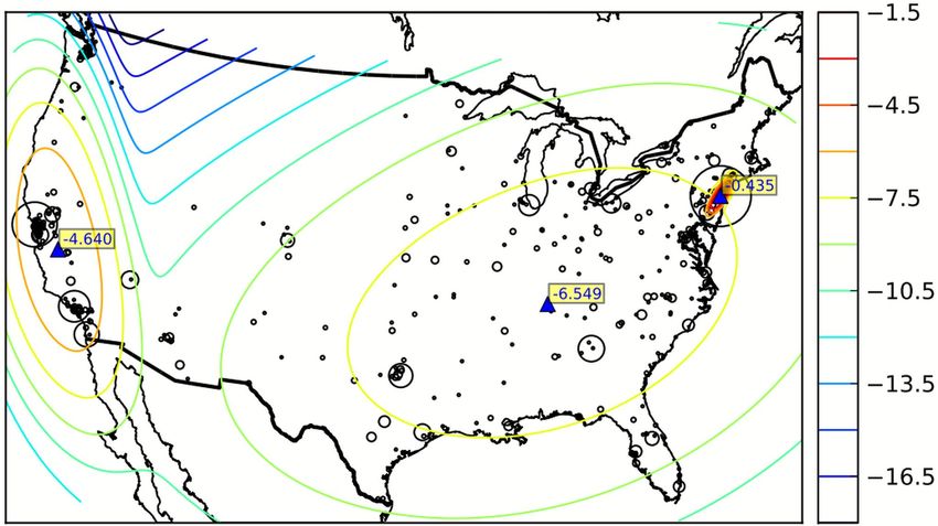
Fig. 2. The occurrences of the stop word for in Twitter data set. use top-k words as the final “local” words to be used in the
prediction.
other words in the data set are local. Despite the promising
results, we believe that such a supervised selection approach B. Finding Local Words by Geometric-Localness: GL
is problematic–i.e., not only their labeling process to manually Intuitively, if a word w has: (1) a smaller number of
create a ground truth is labor intensive and subject to human cities with high probability scores (i.e., only a few peaks),
bias, it is hard to transfer labeled words to new domain or data and (2) smaller average inter-city geometric distances among
set. Moreover, the dictionary used in labeling process might those cities with high probability scores (i.e., geometrically
not differentiate the evidences on different forms of a word. clustered), then one can view w as a local word. That is, a
For example, the word bears (i.e., name of an NFL team) is local word should have a high probability density clustered
likely to be a local word, while the word bear might not be. within a small area. Therefore, based on these observations,
As a result, we believe that a better approach is to automate we propose the Geometric-Localness, GL, of a word w:
the process (i.e., unsupervision) such that the decision on the
P (c0i |w)
P
localness of a word is made only by their actual spatial word c0i ∈C 0
usage, rather than their semantic meaning being interpreted by GL(w) = P
geo-dist(cu ,cv )
human labelers. Toward this challenge, in the following, we |C 0 |2 |{(c u ,cv )}|
propose two unsupervised methods to select a set of “local where geo-dist(cu , cv ) measures the geometric distance in
words” from a corpus using the evidences from tweets and miles between two cities cu and cv . Suppose one sort cities
their tweeter locations directly. c (∈ C) according to P (c|w). Using a user-set threshold
A. Finding Local Words by Non-Localness: N L parameter, r (0 < r < 1), then, one can find a sub-list
of cities C 0 = (c01 , ..., c0|C 0 | ) s.t. P (c0i |w) ≥ P (c0i+1 |w) and
Stop words such as the, you, or for are in general P 0
c0i ∈C 0 P (ci |w) ≥ r. In the formula of GL(w), the numerator
commonly used words that bear little significance and con- then favors words with a few “peaky” cities whose aggregated
sidered as noises in many IR applications such as search probability scores satisfy the threshold r. The denominator in
engine or text mining. For instance, compare Fig. 2 showing turn indicates that GL(w) score is inversely proportional to the
the frequency distribution for the stop word for to Fig. 1 number of “peaky” cities (i.e., |C 0 |2 ) and their average inter-
showing that for word with strong local usage pattern like
P
geo-dist(cu ,cv )
distance (i.e., |{(cu ,cv )}| ). From the initial tweet message
giants. In Fig. 2, one is hard to pinpoint a few hotspot
corpus, finally, we rank each word wi by its GL(wi ) score
locations for for since it is globally used.In the location
in descending order and use top-k words as the final “local”
prediction task, as such, the spatial word usage of these stop
words to be used in the prediction.
words shows a somewhat uniform distributions adjusted to
the sampled data set. As an automatic way to filter noisy V. E XPERIMENTAL VALIDATION
non-local words out from the given corpus, therefore, we A. Set-Up
propose to use the stop words as counter examples. That
is, local words tend to have the farthest distance in spatial For validating the proposed ideas, we used the same Twitter
word usage pattern to stop words. We first estimate a spatial data set collected and used by [3]. This data set was originally
word usage p(C|w) for each word as well as stop words. collected between Sep. 2009 and Jan. 2010 by crawling
The similarity of two words, wi and wj , can be measured by through Twitter’s public timeline API as well as crawling
the distance between two probability distributions, p(C|wi ) by breadth-first search through social edges to crawl each
and p(C|wj ). We consider two divergences for measuring the user’s followees/followers. The data set is further split into
distance: Symmetric Kullback-Leibler divergence (simSKL ) training and test sets. The training set consists of users whose
and Total Variation (simT V ): location is set in city levels and within the US continental,
resulting in 130,689 users with 4,124,960 tweets. The test set
X P (c|wi ) P (c|wj ) consists of 5,119 active users with around 1,000 tweets from
simSKL (wi , wj ) = P (c|wi ) ln + P (c|wj ) ln
c∈C
P (c|wj ) P (c|wi ) each, whose location is recorded as a coordinate (i.e., latitude
and longitude) by GPS device, a much more trustworthy data
X
simT V (wi , wj ) = |P (c|wi ) − P (c|wj )|
c∈C than user-edited location information. In our experiments, weTABLE I 0.5
BASELINE RESULTS USING DIFFERENT MODELS . 1100
0.4
PProbability
P Model ACC AED
0.3
900
(1) P P log(P (c|wi )P (wi )) 0.1045 1,760.4
(2) P P P (c|wi )P (wi ) 0.1022 1,768.73 700
0.2
(3) log P (wi |c) 0.1914 1,321.42
Model (1), SKL
Model (1), SKL
Model (2), SKL
Model (2), SKL 500
0.1 Model (3), SKL Model (3), SKL
TABLE II Model (1), TV Model (1), TV
Model (2), TV Model (2), TV
R ESULTS OF M ODEL (1) ON GMM WITH VARYING # OF COMPONENTS K. 0
Model (3), TV
300
Model (3), TV
1K 2K 3K 4K 5K 6K 1K 2K 3K 4K 5K 6K
K 1 2 3 4 5 (a) ACC (b) AED
ACC 0.0018 0.025 0.3188 0.2752 0.2758
AED 958.94 1785.79 700.28 828.71 826.1 Fig. 3. Results with local words selected by Non-Localness (NL) on MLE
K 6 7 8 9 10 estimation (X-axis indicates # of top-k local words used).
ACC 0.2741 0.2747 0.2739 0.2876 0.3149
AED 830.62 829.14 830.33 786.34 746.75
GMM shows much improvements over baseline results of
Table I. Table II shows the results using Model (1) whose
considered only 5,913 US cities with more than 5,000 of probabilities are estimated by GMM with different # of
population in Census 2000 U.S. Gazetteer. Therefore, the components K, using all the words in the corpus. Except the
problem that we experimented is to correctly predict one cases with K = 1 and K = 2, all GMM based estimations
city out of 5,913 candidates as the home location of each show substantial improvements over MLE based ones, where
Twitter user. We preprocess the training set by removing non- the best ACC (0.3188) and AED (700.28 miles) are achieved
alphabetic characters (e.g., “@”) and stop words, and selects at K = 3. Although the actual # of locations of interests
the words of at least 50 occurrences, resulting in 26,998 varies for each word, in general, we believe that the words
unique terms at the end in our dictionary. No stemming that have too many location of interests are unlikely to make
is performed since singular and plural forms may provide contribution to the prediction. That is, as K becomes large,
different evidences as discussed in Section IV. Data sets and the probabilities are more likely to be distributed, thus making
codes that we used in the experiments are publicly available the prediction harder. Therefore, in subsequent experiments,
at: http://pike.psu.edu/download/asonam12/. we focus on GMM with a small # of components.
To measure the effectiveness of estimating user’s home
location, we used the following two metrics also used in the D. Prediction with Unsupervised Selection of Local Words
literature [3], [2], [11]. First, the accuracy (ACC) measures
We attempt to see if the “local words” idea first proposed
the average fraction of successful estimations for the given
in [3] can be validated even when local words are selected
user set U : ACC = |{u|u∈U and dist(Loc|U true (u),Locest (u))≤d}|
| .
in the unsupervised fashion (as opposed to [3]’s supervised
The successful estimation is defined as when the distance of
approach). In particular, we validate with two unsupervised
estimated and ground-truth locations is less than a threshold
methods that we proposed on MLE estimation.
distance d. Like [3], [2], we use d = 100 (miles) as the
threshold. Second, for understanding the overall margins of 1) Non-Localness (NL): In measuring N L(w) score of a
errors, we use the average error distance (AED) as: AED = word w, we use the English stop word list from SMART
system [10]. A total of 493 stop words (out of 574 in the
P
u∈U dist(Loctrue (u),Locest (u))
|U | .
B. Baselines original list), roughly 1.8% of all terms in our dictionary,
occurred about 23M times (52%) in the training data. Due to
In Section 2, we compared three different models as their common uses in the corpus, such stop words are viewed
discussed in Sec II to understand the impact of selecting as the least indicative of user locations. Therefore, N L(w)
the underlying probability frameworks. Table I presents the measures the degree of similarity of w to average probability
results of different models for location estimation. All the distributions of 493 stop words. Accordingly, if w shows the
probabilities are estimated with MLE using all words in our most dissimilar spatial usage pattern, i.e. P (C|w), from those
dictionary. The baseline Models (1) and (2) (proposed by [3]) of stop words, then w is considered to be a candidate local
utilize the spatial word usage idea, and have around 0.1 of word. The ACC and AED (in miles) results are shown in
ACC and around 1,700 miles in AED. The Model (3), a Fig. 3, as a function of the # of local words used (i.e., chosen
language model approach, shows a much improved result– as top-k when sorted by N L(w) scores). In summary, Model
about two times higher ACC and AED with 400 miles less. (2) shows the best result of ACC (0.43) and AED (628 miles)
These results are considered as baselines in our experiments. with 3K local words used, a further improvement over the
C. Prediction with GMM Based Estimation best result by GMM in Section V-C of ACC (0.3188) and
Next, we study the impact of the proposed GMM estima- AED (700.28 miles). Model (1) has a better ACC but a worse
tion1 for estimating locations. In general, the results using AED than Model (3) has. In particular, local words chosen
using simT V as the similarity measure outperforms simSKL
1 Using EM implementation from scikit-learn, http://scikit-learn.org for all three Models.0.5 0.5 1000
Model (1), SKL
Model (2), SKL
1100 900 Model (1), TV
0.4 0.4 Model (2), TV
800
900 0.3
0.3 700
600
0.2 700 0.2
Model (1), r=0.1 500
Model (1), r=0.1
Model (2), r=0.1 Model (1), SKL
Model (2), r=0.1 500 0.1
0.1 Model (3), r=0.1 Model (3), r=0.1 Model (2), SKL 400
Model (1), r=0.5 Model (1), r=0.5 Model (1), TV
Model (2), r=0.5 Model (2), r=0.5 Model (2), TV
Model (3), r=0.5 Model (3), r=0.5 0 300
0 300
1K 2K 3K 4K 5K 6K 1K 2K 3K 4K 5K 6K
1K 2K 3K 4K 5K 6K 1K 2K 3K 4K 5K 6K
(a) ACC, r = 0.1, 0.5 (b) AED, r = 0.1, 0.5 (a) ACC (b) AED
0.5 1100
Fig. 5. Results with local words selected by Non-Localness (NL) on GMM
estimation (X-axis indicates # of top-k local words used).
0.4
900
TABLE III
0.3 E XAMPLES OF CORRECTLY ESTIMATED CITIES AND CORRESPONDING
700 TWEET MESSAGES ( LOCAL WORDS ARE IN BOLD FACE ).
0.2
Est. City Tweet Message
Model (1), TOP 2K Model (1), TOP 2K
0.1
Model (2), TOP 2K 500
Model (2), TOP 2K
i should be working on my monologue for my au-
Model (3), TOP 2K Model (3), TOP 2K
Model (1), TOP 3K Model (1), TOP 3K Los Angeles dition thursday but the thought of memorizing some-
Model (2), TOP 3K Model (2), TOP 3K
0
Model (3), TOP 3K
300 Model (3), TOP 3K thing right now is crazy
0.1 0.2 0.3 0.4 0.5 0.6 0.7 0.8 0.9 0.1 0.2 0.3 0.4 0.5 0.6 0.7 0.8 0.9 i knew deep down inside ur powell s biggest fan p
lakers will win again without kobe tonight haha if
(c) ACC, # word=2K, 3K (d) AED, # word=2K, 3K Los Angeles
morisson leaves lakers that means elvan will not be
Fig. 4. Results with local words selected by Geometric-Localness (GL) on rooting for lakers anymore
MLE estimation (X-axis in (a) and (b) indicates # of top-k local words used the march vogue has caroline trentini in some awe-
and that in (c) and (d) indicates r of GL(w) formula). some givenchy bangles i found a similar look for less
New York
an intern from teen vogue fashion dept just e mailed
me asking if i needed an assistant aaadorable
2) Geometric-Localness (GL): Our second approach selects
a word w as a local word if w yields only a small number
P (C|W ), GMM based estimation cannot be used for Model
of cities with high probability scores (i.e., only a few peaks)
(3), and thus is not compared. Due to the limitation of space,
and a smaller average inter-city geometric distances. Fig. 4(a)
we report the best case using N L(w) in Fig 5. Model (1)
and (b) show the ACC and AED of three probability models
generally outperforms Model (2) and achieves the best result
P either r = 0.1 and r = 0.5. The user-set parameter r
using
so far for both ACC (0.486) and AED (583.2 miles) with
(= c0 ∈C 0 P (c0i |w)) of GL(w) formula indicates the sum of
i simT V using 2K local words. While details are omitted, it is
probabilities of top candidate cities C 0 . Overall, all variations
worthwhile to note that when used together with GMM, N L
show similar behavior, but in general, Model (2) based vari-
in general outperforms GL, unlike when used with MLE.
ations outperform Model (1) or (3) based ones. Model (2) in
Table III illustrates examples where cities are predicted
particular achieves the best performance of ACC (0.44) and
successfully by using N L-selected local words and with
AED (600 miles) with r = 0.5 and 2K local words. Note that
GMM-based estimation. Note that words such as audition
this is a further improvement over the previous case using
(i.e., the Hollywood area is known for movie industries) and
N L as the automatic method to pick local words–ACC (0.43)
kobe (i.e., name of the basketball player based in the area)
and AED (628 miles) with 3K local words. Fig. 4(c) and (d)
are a good indicator of the city of the Twitter user.
show the impact of r in GL(w) formula, in X-axis, with the
In summary, overall, Model (1) shows a better performance
number of local words used fixed at 2K and 3K. In general,
with GMM while Model (2) with MLE as the estimation
GL shows the best results when r is set to the range of 0.4
model. In addition, Model (1) usually uses less words to
– 0.6. In particular, Model (2) is more sensitive to the choice
reach the best performance than Model (2) does. In terms of
of r than Models (1) and (3). In general, we found that GL
selecting local words, N L works better than GL in general,
slightly outperforms N L in both ACC and AED metrics.
with simT V in particular. In contrast, the best value of r
E. Prediction with GMM and Local Words depends on the model and the estimation method used. The
best result for each model is summarized in Table IV while
In previous two sub-sections, we show that both GMM
further details on different combinations of those best results
based estimation with all words and MLE based estimation
for Models (1) and (2) are shown Fig. 6.
with unsupervised local word selection are effective, compared
to baselines. Here, further, we attempt to improve the result
by combining both approaches to have unsupervised local TABLE IV
word selection on the GMM based estimation. We first use S UMMARY OF BEST RESULTS OF PROBABILITY AND ESTIMATION MODELS .
the GMM to estimate P (C|w) with K = 3, and calculate
Model Estimation Measure Factor #word ACC AED
both N L(w) and GL(w) using P (C|w). Finally, we use the (1) GMM NL simT V 2K 0.486 583.2
top-k local words and their P (C|w) to predict user’s location. (2) MLE GL r = 0.5 2K 0.449 611.6
Since Model (3) makes a prediction with P (W |C) rather than (3) MLE GL r = 0.1 2.75K 0.323 827.80.5 0.5 TABLE V
P REDICTION WITH REDUCED # OF LOCAL WORDS BY FREQUENCY.
0.4 0.4
(a) Model (1), GMM, N L
0.3 0.3
Number of local words used
0.2 0.2 50 100 150 200 250
GL, MLE, r=0.4 GL, MLE, r=0.5 Top 2K 0.433 0.447 0.466 0.476 0.499
0.1
NL, MLE, TV
0.1
NL, MLE, TV ACC
GL, GMM, r=0.1 GL, GMM, r=0.1 Top 3K 0.446 0.449 0.444 0.445 0.446
NL, GMM, TV NL, GMM, TV
Baseline Baseline Top 2K 603.2 599.6 582.9 565.7 531.1
0 0 AED
1K 2K 3K 4K 5K 6K 1K 2K 3K 4K 5K 6K Top 3K 509.3 567.7 558.9 539.9 536.5
(a) Model (1) (b) Model (2) (b) Model (1), MLE, GL
Fig. 6. Settings for two models to achieve the best ACC. Number of local words used
50 100 150 200 250
F. Smoothing vs. Feature Selection Top 2K 0.354 0.382 0.396 0.419 0.420
ACC
Top 3K 0.397 0.400 0.399 0.403 0.416
The technique to simultaneously increase the probability Top 2K 771.7 761.0 760.3 730.6 719.8
of unseen terms (that cause the sparseness problem) and AED
Top 3K 806.2 835.1 857.5 845.9 822.3
decrease that of seen terms is referred to as smoothing. While
(c) Model (3), MLE, GL
successfully applied in many IR problems, in the context of
location prediction problem from Twitter data, it has been Number of local words used
50 100 150 200 250
reported that smoothing has very little effect in improving
Top 2K 0.2227 0.276 0.315 0.336 0.343
the accuracy [11], [3]. On the other hand, as reported in [3], ACC
Top 3K 0.301 0.366 0.385 0.401 0.408
feature selection seems to be very effective in solving the AED
Top 2K 743.9 663.3 618.5 577.7 570.3
location prediction problem. That is, instead of using the Top 3K 620.7 565.6 535.1 510.8 503.3
entire corpus, [3] proposed to use a selective set of “local
words” only. Through the experiments, we validated that the However, again, their overall impact is very limited due to the
feature selection idea via local words is indeed effective. For rarity outside those towns. From these observations, therefore,
instance, Fig. 6 shows that our best results usually occur we believe that both localness as well as frequency information
when around 2,000 local words (identified by either N L or of words must be considered in ranking local words.
GL methods), instead of 26,998 original terms, are used in Informally, score(w) = λ localness(w)
∆l + (1 − λ) frequency(w)
∆f ,
predicting locations. Having a reduced feature set is beneficial, where ∆l and ∆f are normalization constants for
especially in terms of speed. For instance, with Model (1) localness(w) and frequency(w) functions, and λ controls
estimated by MLE, using 50, 250, 2,000, and 26,999 local the relative importance between localness and frequency of
words, it took 27, 32, 50, and 11,531 seconds respectively to w. The localness of w can be calculated by either N L or
finish the prediction task. In general, if one can get comparable GL, while frequency of w can be done using IR methods
results in ACC and AED, solutions with a smaller feature set such as relative frequency or TF-IDF. For simplicity, in
(i.e., less number of local words) are always preferred. As this experiments, we implemented the score() function in
such, in this section, we report our exploration to reduce the two-steps: (1) we first select base 2,000 or 3,000 local words
number of local words used in the estimation even further. by N L or GL method; and (2) next, we re-sort those local
Figs. 4–6 all indicate that both ACC and AED (in all words based on their frequencies. Table V shows the results
settings) improve in proportion to the size of local words up to of ACC and AED using only a small number (i.e., 50–250) of
2K–3K range, but deviate afterwards. In particular, note that top-ranked local words after re-sorted based on both localness
those high-ranked words within top-300 (according to N L or and frequency information of words. Note that using only
GL measures) may be good local words but somehow have 50–250 local words, we are able to achieve comparable ACC
limited impact toward overall ACC and AED. For instance, and AED to the best cases of Table IV that use 2,000–3,000
using GMM as the estimation model, GL yields the follow- local words. The improvement is the most noticeable for
ing within the top-10 local words: {windstaerke, prazim, Model (1). The results show the quality of the location
cnen}. Upon inspection, however, these words turn out to prediction task may rely on a small set of frequently-used
be Twitter user IDs. These words got high local word scores local words.
(i.e., GL) probably because their IDs were used in re-tweets Table VI shows top-30 local words with GMM, when re-
or mentioned by users with a strong spatial pattern. Despite sorted by frequency, from 3,000 N L-selected words. Note that
their high local word scores, however, their usage in the entire most of these words are toponyms, i.e., names of geographic
corpus is relatively low, limiting their overall impact. Similarly, locations, such as nyc, dallas, and fl. Others include the
using MLE as the estimation mode, N L found the followings names of people, organizations or events that show a strong
at high ranks: {je, und, kt}. These words are Dutch (thus not local pattern with frequent usage, such as obama, fashion,
filtered in preprocessing) and heavily used in only a few US or bears. Therefore, it appears that toponyms are important
towns2 of Dutch descendants, thus exhibiting a strong locality. in predicting the locations of Tweeter users. Interestingly, a
previous study in [11] showed that toponyms from image
2 Nederland (Texas), Rotterdam (New York), and Holland (Michigan) tags were helpful, though not significantly, in predicting theTABLE VI 0.8
←default setting
0.5 1000
T OP -30 F REQUENCY- RESORTED LOCAL WORDS (GMM, N L).
0.4
0.6
800
la nyc hiring dallas francisco
AED (miles)
0.3
obama fashion atlanta houston denver
ACC
0.4
san diego sf austin est 0.2
chicago los seattle hollywood yankees 600
0.2
york boston washington angeles bears 0.1
ny miami dc fl orlando Model(1) GMM NL 2000 250 Model(1) GMM NL 2000 250 Model(1) GMM NL 2000 250
Model(1) GMM NL 3000 50 Model(1) GMM NL 3000 50 Model(1) GMM NL 3000 50
0 0 400
100 250 500 750 1000 10% 20% 40% 60% 80% 100%
TABLE VII Distance threshold d (miles) % of tweets used per user
P REDICTION WITH ONLY TOPONYMS . (a) Varying d (b) Varying |Tu |
Number of toponyms used
Fig. 7. Change of ACC and AED as a function of d and |Tu |.
50 200 400
Model (1) 0.246 0.203 0.115
ACC Model (2) 0.306 0.291 0.099 prediction. We show that our approach can, using less than
Model (3) 0.255 0.347 0.330 250 local words selected by proposed methods, achieve a com-
Model (1) 1202.7 1402.7 1719.7 parable or better performance to the state-of-the-art that uses
AED Model (2) 741.9 953.5 1777.4
Model (3) 668.2 512.4 510.1
3,183 local words (selected by the supervised classification
based on 11,004 hand-labeled ground truth).
location of the images. Table VII shows the results using city ACKNOWLEDGMENT
names with the highest population in U.S. gazetteer as the
“only” features for predicting locations (without using other The research was in part supported by NSF DUE-0817376 and
local words). Note that performances are all improved with all DUE-0937891, and Amazon web service grant (2011). We thank
three models, but are not good as those in Table V. Therefore, Zhiyuan Cheng (infolab at TAMU) for providing their dataset and
we conclude that using toponyms in general improve the feedbacks on their implementation.
prediction of locations, but not all toponyms are equally R EFERENCES
important. Therefore, it is important to find critical local words [1] L. Backstrom, J. Kleinberg, R. Kumar, and J. Novak, “Spatial variation
in search engine queries,” in WWW, Beijing, China, 2008, pp. 357–366.
or toponyms using our proposed N L or GL selection methods. [2] S. Chandra, L. Khan, and F. B. Muhaya, “Estimating twitter user location
It further justifies that such a selection needs to be made from using social interactions-a content based approach,” in IEEE SocialCom,
the evidences in tweet contents and user location, rather based 2011, pp. 838–843.
[3] Z. Cheng, J. Caverlee, and K. Lee, “You are where you tweet: a content-
on semantic meanings or types of words (as [3] did). based approach to geo-locating twitter users,” in ACM CIKM, Toronto,
ON, Canada, 2010, pp. 759–768.
G. Discussion on Parameter Settings [4] N. Dalvi, R. Kumar, and B. Pang, “Object matching in tweets with
First, same as the setting in literature, we used d = 100 spatial models,” in ACM WSDM, Seattle, Washington, USA, 2012, pp.
43–52.
(miles) in computing ACC–i.e., if the distance between the [5] B. Hecht, L. Hong, B. Suh, and E. H. Chi, “Tweets from justin bieber’s
estimated city and ground truth city is less than 100 miles, heart: the dynamics of the location field in user profiles,” in ACM CHI,
we consider the estimation to be correct. Fig. 7(a) shows that Vancouver, BC, Canada, 2011, pp. 237–246.
[6] P. Kelm, S. Schmiedeke, and T. Sikora, “Multi-modal, multi-resource
ACC as a function of d using the best configuration (Model methods for placing flickr videos on the map,” in ACM Int’l Conf. on
(1), GMM, N L) with 50 and 250 local words, respectively. Multimedia Retrieval (ICMR), Trento, Italy, 2011, pp. 52:1–52:8.
Second, the test set that we used in experiments consists of [7] S. Kinsella, V. Murdock, and N. O’Hare, ““i’m eating a sandwich in
glasgow”: modeling locations with tweets,” in Int’l workshop on Search
a set of active users with around 1K tweets, same setting and Mining User-Generated Contents (SMUC), Glasgow, Scotland, UK,
as [3] for comparison. Since not all Twitter users have that 2011, pp. 61–68.
many tweets, we also experiment using different portion of [8] M. Larson, M. Soleymani, P. Serdyukov, S. Rudinac, C. Wartena,
V. Murdock, G. Friedland, R. Ordelman, and G. J. F. Jones, “Automatic
tweet messages per user. That is, per each user in the test set, tagging and geotagging in video collections and communities,” in ACM
we randomly select from 1% to 90% of tweet messages to Int’l Conf. on Multimedia Retrieval (ICMR), Trento, Italy, 2011, pp.
predict locations. The average results from 10 runs are shown 51:1–51:8.
[9] W. Li, P. Serdyukov, A. P. de Vries, C. Eickhoff, and M. Larson, “The
in Fig. 7(b). While we achieve ACC (shown in left Y-axis) where in the tweet,” in ACM CIKM, Glasgow, Scotland, UK, 2011, pp.
of 0.104 using 1% (10 tweets) per user, it rapidly improves 2473–2476.
to 0.2 using 3% (30 tweets), and 0.3 using 7% (70 tweets). [10] G. Salton, The SMART Retrieval System - Experiments in Automatic
Document Processing. Upper Saddle River, NJ, USA: Prentice-Hall,
Asymmetrically, AED (shown in right Y-axis) decreases as Inc., 1971.
tweets increases. [11] P. Serdyukov, V. Murdock, and R. van Zwol, “Placing flickr photos on
a map,” in ACM SIGIR, Boston, MA, USA, 2009, pp. 484–491.
VI. C ONCLUSION [12] O. Van Laere, S. Schockaert, and B. Dhoedt, “Finding locations of flickr
resources using language models and similarity search,” in ACM Int’l
In this paper, we aim to improve the quality of predicting Conf. on Multimedia Retrieval (ICMR), Trento, Italy, 2011, pp. 48:1–
Twitter user’s home location under probability frameworks. 48:8.
[13] C. Zhai and J. Lafferty, “A study of smoothing methods for language
We proposed a novel approach to estimate the spatial word models applied to information retrieval,” ACM Trans. Inf. Syst., vol. 22,
usage probability with Gaussian Mixture Models. We also no. 2, pp. 179–214, Apr. 2004.
proposed unsupervised measurements to rank the local words
which effectively remove the noises that are harmful to theYou can also read