Positive, Negative, or Neutral: Learning an Expanded Opinion Lexicon from Emoticon-Annotated Tweets
←
→
Page content transcription
If your browser does not render page correctly, please read the page content below
Proceedings of the Twenty-Fourth International Joint Conference on Artificial Intelligence (IJCAI 2015)

                           Positive, Negative, or Neutral: Learning an Expanded
                            Opinion Lexicon from Emoticon-Annotated Tweets

                        Felipe Bravo-Marquez, Eibe Frank and Bernhard Pfahringer
                            Department of Computer Science, University of Waikato
                             fjb11@students.waikato.ac.nz, {eibe,bernhard}@waikato.ac.nz

                               Abstract                                           apple will receive different sentiment scores when used to re-
                                                                                  fer to a common noun (a fruit) or a proper noun (a company).
         We present a supervised framework for expanding                             The proposed methodology takes a stream of tweets noisily
         an opinion lexicon for tweets. The lexicon contains                      labelled according to their polarity using emoticon-based an-
         part-of-speech (POS) disambiguated entries with a                        notation. In this approach, only tweets with positive or neg-
         three-dimensional probability distribution for pos-                      ative emoticons are considered and labelled according to the
         itive, negative, and neutral polarities. To obtain                       polarity indicated by the emoticon. This idea has been widely
         this distribution using machine learning, we pro-                        used before to train message-level sentiment classifiers [Bifet
         pose word-level attributes based on POS tags and                         and Frank, 2010], [Go et al., 2009].
         information calculated from streams of emoticon-
                                                                                     We calculate two types of word-level attributes from the
         annotated tweets. Our experimental results show
                                                                                  stream of annotated tweets to train a word classifier: Seman-
         that our method outperforms the three-dimensional
                                                                                  tic Orientation (SO) [Turney, 2002], which is based on the
         word-level polarity classification performance ob-
                                                                                  mutual information between word and sentiment class, and
         tained by semantic orientation, a state-of-the-art
                                                                                  Stochastic Gradient Descent (SGD) score, which learns a lin-
         measure for establishing world-level sentiment.
                                                                                  ear relationship between word and sentiment class. Addition-
                                                                                  ally, we consider syntactic information of the word in its con-
1       Introduction                                                              text by including the POS tag of the word as a nominal at-
                                                                                  tribute.
The language used in Twitter1 provides substantial chal-
                                                                                     To train a word-level sentiment classifier using supervised
lenges for sentiment analysis. The words used in this plat-
                                                                                  learning, we also need sentiment labels for the words. These
form include many abbreviations, acronyms, and misspelled
                                                                                  labels are provided by a seed lexicon taken from the union of
words that are not observed in traditional media or covered
                                                                                  four different hand-made lexicons after discarding all polarity
by popular lexicons. The diversity and sparseness of these in-
                                                                                  clashes from the intersection.
formal words make the manual creation of a Twitter-oriented
opinion lexicon a time-consuming task.                                               To the best of our knowledge, this is the first article in
   In this article we propose a supervised framework for opin-                    which the lexicon expansion of Twitter opinion words using
ion lexicon expansion for the language used in Twitter. Tak-                      POS disambiguation and supervised learning is studied and
ing SentiWordnet as inspiration, each word in our expanded                        evaluated. Additionally, this is the first study in which scores
lexicon has a probability distribution, indicating how positive,                  for positive, negative, and neutral sentiment are provided for
negative, and neutral it is. The estimated probabilities can be                   Twitter-specific expressions.
used to represent intensities for a specific sentiment category                      We test our approach on two collections of automatically
e.g., the word awesome is more positive than the word ade-                        labelled tweets. The results indicate that our supervised
quate. Furthermore, the neutral dimension may be useful for                       framework outperforms semantic orientation when the de-
discarding non-opinion words in text-level polarity classifica-                   tection of neutral words is considered. We also evaluate the
tion tasks. In contrast, unsupervised lexicon expansion tech-                     usefulness of the expanded lexicon for message-level polarity
niques such as semantic orientation [Turney, 2002] provide a                      classification of tweets, showing significant improvements in
single numerical score for each word, and it is unclear how to                    performance.
impose thresholds on this score for neutrality detection.                            This article is organised as follows. In Section 2 we pro-
   All the entries in our lexicon are associated with a cor-                      vide a review of existing work in opinion lexicon expansion.
responding part-of-speech tag. By relying on POS-tagged                           In Section 3 we describe the seed lexicon used to label the
words, homographs2 with different POS-tags will be disam-                         words for the training set. In Section 4 we explain the mech-
biguated [Wilks and Stevenson, 1998]. For instance, the word                      anisms studied to automatically create collections of labelled
                                                                                  tweets. The creation of our word-level time-series is de-
    1
        http://www.twitter.com                                                    scribed in Section 5, together with the features used for train-
    2
        Words that share the same spelling but have different meanings.           ing the classifier. In Section 6 we present the experiments

                                                                           1229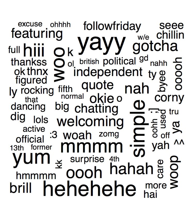
we conducted to evaluate the proposed approach and discuss                 3       Ground-Truth Word Polarities
results. The main findings and conclusions are discussed in
Section 7.                                                                 In this section, we describe the seed lexicon used to label the
                                                                           training dataset for our word sentiment classifier. We create it
2       Related Work                                                       by taking the union of the following manually created lexical
                                                                           resources:
There are two types of resources that can be exploited for
                                                                              MPQA Subjectivity Lexicon: This lexicon was created by
lexicon expansion: thesauri and document collections. The
                                                                           Wilson et al. [Wilson et al., 2005] and is part of Opinion-
simplest approach using a thesaurus such as WordNet3 is to
                                                                           Finder5 , a system that automatically detects subjective sen-
expand a seed lexicon of labelled opinion words using syn-
                                                                           tences in document corpora. The lexicon has positive, nega-
onyms and antonyms from the lexical relations provided by
                                                                           tive, and neutral words.
the thesaurus [Hu and Liu, 2004], [Kim and Hovy, 2004].
The hypothesis behind this approach is that synonyms have                     Bing Liu: This lexicon is maintained and distributed by
the same polarity and antonyms have the opposite. This pro-                Bing Liu6 and was used in several of his papers [Liu, 2012].
cess is normally iterated several times. In [Esuli and Sebas-              It has positive and negative entries.
tiani, 2005], a supervised classifier was trained using a seed                Afinn: This strength-oriented lexicon [Nielsen, 2011] has
of labelled words that was obtained through synonyms and                   positive words scored from 1 to 5 and negative words scored
antonyms expansion. For each word, a vector space model is                 from -1 to -5. It includes slang, obscene words, acronyms
created from the definition or gloss provided by the WordNet               and Web jargon. We tagged words with negative and positive
dictionary. This representation is used to train a word-level              scores to negative and positive classes respectively.
classifier that is used for lexicon expansion. An equivalent                  NRC emotion Lexicon: This emotion-oriented lexicon
approach was applied later to create SentiWordnet4 in [Esuli               [Mohammad and Turney, 2013] was created by conducting
and Sebastiani, 2006], [Baccianella et al., 2010]. In Senti-               a tagging process on the crowdsourcing Amazon Mechani-
WordNet, each WordNet synset or group of synonyms is as-                   cal Turk platform. In this lexicon, the words are annotated
signed into classes positive, negative and neutral in the range            according to eight emotions: joy, trust, sadness, anger, sur-
[0, 1].                                                                    prise, fear, anticipation, and disgust, and two polarity classes:
   A limitation of thesaurus-based approaches is their inabil-             positive and negative. There are many words that are not as-
ity to capture domain-dependent words. Corpus-based ap-                    sociated with any emotional state and are tagged as neutral.
proaches exploit syntactic or co-occurrence patterns to ex-                In this work, we consider positive, negative, and neutral tags
pand the lexicon to the words found within a collection of                 from this lexicon.
documents. In [Turney, 2002], the expansion is done through                   As we need to reduce the noise in our training data, we dis-
a measure referred to as semantic orientation, which is based              card all words where a polarity clash is observed. A polarity
on the the point-wise mutual information (PMI) between two                 clash is a word that receives two or more different tags in the
random variables:                                                          union of lexicons. The number of words for the different po-
                                                                           larity classes in the different lexicons is displayed in Table 1.

                                    P r(term1 ∧ term2 )
   PMI(term1 , term2 ) = log2
                                   P r(term1 )P r(term2 )
                                                              (1)                                      Positive    Negative    Neutral
   The semantic orientation of a word is the difference be-                          AFINN               564         964         0
tween the PMI of the word with a positive emotion and a                              Bing Liu           2003        4782         0
negative emotion. Different ways have been proposed to rep-                          MPQA               2295        4148        424
resent the joint probabilities of words and emotions. In Tur-                        NRC-Emo            2312        3324        7714
ney’s work [Turney, 2002], they are estimated using the num-                         Seed Lexicon       3730        6368        7088
ber of hits returned by a search engine in response to a query
composed of the target word together with the word “excel-
                                                                                                Table 1: Lexicon Statistics
lent” and another query using the word “poor”.
   The same idea was used for Twitter lexicon expansion
in [Becker et al., 2013], [Mohammad et al., 2013], [Zhou et                   From the table, we can observe that the number of words
al., 2014], which all model the joint probabilities from col-              per class is significantly reduced after removing the clashes
lections of tweets labelled in automatic ways. In [Becker et               from the union. The total number of clashes is 1074.
al., 2013], the tweets are labelled with a trained classifier us-             This high number of clashes found among different hand-
ing thresholds for the different classes to ensure high preci-             made lexicons indicates two things: 1) Different human an-
sion. In [Zhou et al., 2014], they are labelled with emoti-                notators can disagree when tagging a word to polarity classes.
cons to create domain-specific lexicons. In [Mohammad et                   2) There are several words that can belong to more than one
al., 2013], they are labelled with emoticons and hashtags as-              sentiment class. Due to this, we can say that word-level po-
sociated with emotions to create two different lexicons. These             larity classification is a hard and subjective problem.
lexicons were tested for tweet-level polarity classification.
    3                                                                          5
        http://wordnet.princeton.edu/                                              http://mpqa.cs.pitt.edu/opinionfinder/opinionfinder 2/
    4                                                                          6
        http://sentiwordnet.isti.cnr.it/                                           http://www.cs.uic.edu/∼liub/FBS/sentiment-analysis.html

                                                                    1230
4 Obtaining Labelled Tweets The variables w, b, and λ correspond to the weight vector,
the bias, and the regularisation parameter, respectively. The
In order to calculate the attributes for our word-level classi-
class labels y are assumed to be in {+1, −1}, correspond-
fier, we require a collection of time-stamped tweets with their
ing to positively and negatively labelled tweets, respectively.
corresponding polarity labels.
The regularisation parameter was set to 0.0001. The model’s
We rely on the emoticon-based annotation approach in weights determine how strongly the presence of a word in-
which tweets exhibiting positive :) and negative :( emoticons fluences the prediction of negative and positive classes [Bifet
are labelled according to the emoticon’s polarity [Go et al., and Frank, 2010]. The SGD time-series is created by apply-
2009]. Afterwards, the emoticon used to label the passage is ing this learning process to a collection of labelled tweets and
removed from the content. storing the word’s coefficients in different time windows. We
We consider two collections of tweets covering multiple use time windows of 1, 000 examples.
topics: The Edinburgh corpus (ED) [Petrović et al., 2010],
The second time-series corresponds to the accumulated se-
and the Stanford Sentiment corpus (STS) [Go et al., 2009].
mantic orientation (SO) introduced in Section 2. Let count be
The ED corpus has 97 million tweets which were collected a function that counts the number of times that a word or a
using the Twitter streaming API in a period spanning Novem- sentiment label has been observed during a certain period of
ber 11th 2009 until February 1st 2010. This collection in- time. We calculate the SO score for each POS-tagged word in
cludes tweets in multiple languages. As was done in [Bifet an accumulated way according to the following expression:
and Frank, 2010], non-English tweets were filtered out, and
tweets without emoticons were discarded.
The STS corpus was created by periodically sending count(word ∧ pos) × count(neg)
queries :) and :( to the Twitter search API between April 6th SO(word) = log2
count(word ∧ neg) × count(pos)
2009 to June 25th 2009. All the tweets in this collection are (3)
written in English. We use time windows of 1, 000 examples and the Laplace
correction to avoid the zero-frequency problem.
ED STS
Positive 1, 813, 705 800, 000 Feature Description
Negative 324, 917 800, 000 mean The mean of the time-series.
Total 2, 138, 622 1, 600, 000 trunc.mean The truncated mean of the time-series.
median The median of the time-series.
last.element The last observation of the time-series.
Table 2: Collection statistics sd The standard deviation of the time-series .
iqr The inter-quartile range.
sg The fraction of times the time-series changes its sign.
The number of tweets for each polarity class in the two sg.diff The sg value for the differenced time-series.
corpora is given in Table 2. We can observe that when using
the streaming API (ED), positive emoticons occur much more Table 3: Time-series features
frequently than negative ones.
We rely on our time-series to extract features that are used
5 Word-level Features to train our world-level polarity classifier. These features
All the tweets from the annotated collection are lowercased, summarise location and dispersion properties of the time-
tokenised and POS-tagged. We use the TweetNLP library series, and are listed in Table 3. Location-oriented features
[Gimpel et al., 2011], which provides a tokeniser and a tag- mean, trimm.mean and median measure the central tendency
ger specifically for the language used in Twitter. We prepend of the time-series. The feature last.element corresponds to the
a POS-tag prefix to each word in order to differentiate homo- last value observed in the time-series. This attribute would be
graphs exhibiting different POS-tags. equivalent to the traditional semantic orientation measure for
To calculate the proposed features, we treat the time-sorted the SO time-series. The features sd, iqr, sg, and sg.diff mea-
collection of tweets as a data stream and create two time- sure the level of dispersion of the time-series.
series for each POS-tagged word observed in the vocabulary: In addition to these time-series features, we include the
the SGD series, and the SO series. These time-series intend POS-tag of the word as a nominal attribute. We include
to capture the evolution of the relationship between a word this attribute based on the hypothesis that non-neutral words
and the sentiment that it expresses. are more likely to exhibit certain POS tags than neutral ones
The first time-series is calculated by incrementally training [Zhou et al., 2014].
a linear support vector machine using stochastic gradient de-
scent (SGD) [Zhang, 2004]. The weights of this linear model 6 Experiments
correspond to POS-tagged words and are updated in an incre-
mental fashion. We optimise the hinge loss function with an In this section, we present our experimental results for Twitter
L2 penalty and a learning rate equal to 0.1: lexicon expansion. In the first part, we study the word-level
polarity classification problem. In the second part, we ex-
λ X pand the seed lexicon using the trained classifier and use it
||w||2 + [1 − y(xw + b)]+ . (2) for message-level polarity classification of tweets.
2
12316.1 Word-level polarity classification also see that POS tags are useful for neutrality detection, but
We calculated the time-series described in Section 5 for the useless for PosNeg. Therefore, we can conclude that positive
most frequent 10, 000 POS-tagged words found in each of our and negative words have a similar distribution of POS tags.
two datasets. The time-series were calculated using MOA7 , a We trained supervised classifiers for the three different
data stream mining framework. classification problems in both datasets STS and ED. The
classification experiments were performed using WEKA8 , a
ED STS machine learning environment. We studied the following
Positive 1027 1023 learning algorithms in preliminary experiments: RBF SVM,
Negative 806 985 Logistic regression, C4.5, and Random Forest. As the RBF
Neutral 1814 1912 SVM produced the best performance among the different
Total 3647 3920 methods, we used this method in our classification experi-
ments with a nested grid search procedure for parameter tun-
ing where internal cross-validation is used to find C and γ.
Table 4: Word-level polarity classification datasets. The evaluation was done using 10 times 10-folds-cross-
validation and different subsets of attributes were compared.
To create training and test data for machine learning, all the All the methods are compared with the baseline of using the
POS-tagged words matching the seed lexicon are labelled ac- last value of the semantic orientation, based on a corrected re-
cording to the lexicon’s polarities. It is interesting to consider sampled paired t-student test with an α level of 0.05 [Nadeau
how frequently positive, negative, and neutral words occur in and Bengio, 2003]. We used the following subsets of at-
a collection of tweets. The number of words labelled as pos- tributes: 1) SO: Includes only the feature SO.last. This is
itive, negative, and neutral for both the ED and STS datasets the baseline and is equivalent to the standard semantic ori-
is given in Table 4. As shown in the table, neutral words are entation measure with the decision boundaries provided by
the most frequent words in both datasets. Moreover, positive the SVM. 2) ALL: Includes all the features. 3)SGD.TS+POS:
words are more frequent than negative ones. Includes all the features from the SGD time-series and the
Next, we focus on the word-level classification problem. POS tag. 4)SO.TS+POS: Includes all the features from the
With the aim of gaining a better understanding of the prob- SO time-series and the POS tag. 5)SO+POS: Includes the
lem, we study three word-level classification problems: features so.last and the POS tag.
1. Neutrality: Classify words as neutral (objective) or non- We evaluate the weighted area under the ROC curves
neutral (subjective). We label positive and negative (AUCs) (to deal with class imbalances) for the four differ-
words as non-neutral for this task. ent subsets of attributes in the two datasets. The classification
results are presented in Table 6. The symbols ◦ and • corre-
2. PosNeg: Classify words to positive or negative classes. spond to statistically significant improvements and degrada-
We remove all neutral words for this task. tions with respect to the baseline, respectively.
3. Polarity: Classify words to classes positive, negative or We can observe a much lower performance in Neutrality
neutral. This is the primary classification problem we detection than in PosNeg. This indicates that the detection
aim to solve. of neutral Twitter words is much harder than distinguishing
We study the information provided by each feature with between positive and negative words. The performance on
respect to the three classification tasks described above. This both datasets tends to be similar. However, the results for
is done by calculating the information gain of each feature. STS are better than for ED. This suggests that a collection
This score is normally used for decision tree learning and of balanced positively and negatively labelled tweets may be
measures the reduction of entropy within each class after per- more suitable for lexicon expansion. Another result is that the
forming the best split induced by the feature. The informa- combination of all features leads to a significant improvement
tion gain obtained for the different attributes in relation to the over the baseline for neutrality and polarity classification. In
three classification tasks is shown in Table 5. The attributes the PosNeg classification task, we can see that the baseline is
achieving the highest information gain per task are marked in very strong. This suggests that SO is very good for discrim-
bold. inating between positive and negative words, but not strong
We can observe that variables measuring the location of the enough when neutral words are included. Regarding SO and
SO and SGD time-series tend to be more informative than the SGD time-series, we can conclude that they are competitive
ones measuring dispersion. Moreover, the information gain for neutrality detection. However, SO-based features are bet-
of these variables is much higher for PosNeg than for neu- ter for PosNeg and Polarity tasks.
trality. SGD and SO are competitive measures for neutrality,
but SO is better for PosNeg. An interesting insight is that
6.2 Lexicon expansion
features that measure the central tendency of the time-series The ultimate goal of the polarity-classification of words is
tend to be more informative than the last values, especially to produce a Twitter-oriented opinion lexicon emulating the
for SGD. These measures smooth the fluctuations of the SGD properties of SentiWordet, i.e., a lexicon of POS-tagged dis-
time-series. We can see that the feature sgd.mean is the best ambiguated entries with their corresponding distribution for
attribute for neutrality classification in both datasets. We can positive, negative, and neutral classes. To do this, we fit a lo-
7 8
http://moa.cs.waikato.ac.nz/ http://www.cs.waikato.ac.nz/ml/weka/
1232Dataset ED STS
Task Neutrality PosNeg Polarity Neutrality PosNeg Polarity
pos-tag 0.062 0.017 0.071 0.068 0.016 0.076
sgd.mean 0.082 0.233 0.200 0.104 0.276 0.246
sgd.trunc.mean 0.079 0.237 0.201 0.104 0.276 0.242
sgd.median 0.075 0.233 0.193 0.097 0.275 0.239
sgd.last 0.057 0.177 0.155 0.086 0.258 0.221
sgd.sd 0.020 0.038 0.034 0.030 0.030 0.052
sgd.sg 0.029 0.000 0.030 0.049 0.017 0.062
sgd.sg.diff 0.000 0.000 0.008 0.005 0.000 0.000
sgd.iqr 0.018 0.012 0.019 0.015 0.014 0.017
so.mean 0.079 0.283 0.219 0.081 0.301 0.232
so.trunc.mean 0.077 0.284 0.215 0.079 0.300 0.229
so.median 0.077 0.281 0.215 0.076 0.300 0.228
so.last 0.069 0.279 0.211 0.084 0.300 0.240
so.sd 0.000 0.015 0.008 0.000 0.012 0.007
so.sg 0.013 0.216 0.126 0.019 0.239 0.142
so.sg.diff 0.000 0.012 0.009 0.000 0.000 0.000
so.iqr 0.000 0.000 0.000 0.000 0.008 0.000
Table 5: Information gain values.
Dataset SO ALL SGD.TS+POS SO.TS+POS SO+POS
ED-Neutrality 0.62 ± 0.02 0.65 ± 0.02 ◦ 0.65 ± 0.02 ◦ 0.65 ± 0.02 ◦ 0.64 ± 0.02 ◦
ED-PosNeg 0.74 ± 0.03 0.75 ± 0.03 0.71 ± 0.03 • 0.74 ± 0.03 0.73 ± 0.03
ED-Polarity 0.62 ± 0.02 0.65 ± 0.02 ◦ 0.64 ± 0.02 0.65 ± 0.02 ◦ 0.64 ± 0.02 ◦
STS-Neutrality 0.63 ± 0.02 0.67 ± 0.02 ◦ 0.66 ± 0.02 ◦ 0.66 ± 0.02 ◦ 0.66 ± 0.02 ◦
STS-PosNeg 0.77 ± 0.03 0.77 ± 0.03 0.75 ± 0.03 • 0.77 ± 0.03 0.77 ± 0.03
STS-Polarity 0.64 ± 0.02 0.66 ± 0.01 ◦ 0.65 ± 0.02 ◦ 0.66 ± 0.02 ◦ 0.66 ± 0.02 ◦
Table 6: World-level classification performance.
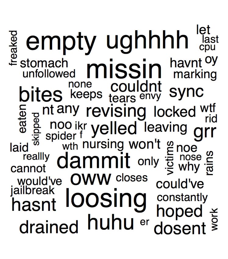
gistic regression model to the output of the support vector ma- sentiment intensities of words. In Figure 1, we visualise
chine trained for the polarity problem using all the attributes. the expanded lexicon intensities of words classified as pos-
The resulting model is then used to classify the remaining un- itive and negative through word clouds. The sizes of the
labelled words. This process is performed for both STS and words are proportional to the log odds ratios log2 ( PP (neg)
(pos)
)
ED datasets.
A sample from the expanded word list is given in Table 7. and log2 ( PP (neg)
(pos) ) for positive and negative words, respec-
We can see that each entry has the following attributes: the tively.
word, the POS-tag, the sentiment label that corresponds to
the class with maximum probability, and the distribution. We
inspected the expanded lexicon and observed that the esti-
mated probabilities are intuitively plausible. However, there
are some words for which the estimated distribution is ques-
tionable, such as the word same in Table 7.
word POS label negative neutral positive
alrighty interjection positive 0.021 0.087 0.892
boooooo interjection negative 0.984 0.013 0.003
lmaoo interjection positive 0.19 0.338 0.472
french adjective neutral 0.357 0.358 0.285
handsome adjective positive 0.007 0.026 0.968
saddest adjective negative 0.998 0.002 0
same adjective negative 0.604 0.195 0.201 (a) (b)
anniversary common.noun neutral 0.074 0.586 0.339
tear common.noun negative 0.833 0.124 0.044 Figure 1: Word clouds of positive and negative words using
relaxing verb positive 0.064 0.244 0.692
wikipedia proper.noun neutral 0.102 0.644 0.254 log odds proportions.
Table 7: Expanded words example.
Next, we study the usefulness of our expanded lexicons
based on ED and STS for Twitter polarity classification. This
The provided probabilities can also be used to explore the involves categorising entire tweets into positive or negative
1233sentiment classes. word-level classification performance shown in Table 6. This
The experiments were performed on three collections of suggests that the two different ways of evaluating the lexicon
tweets that were manually assigned to positive and negative expansion, one at the word level and the other at the message
classes. The first collection is 6HumanCoded9 , which was level, are consistent with each other.
used to evaluate SentiStrength [Thelwall et al., 2012]. In this
dataset, tweets are scored according to positive and negative
numerical scores. We use the difference of these scores to
7 Conclusions
create polarity classes and discard messages where it is equal In this article, we presented a supervised method for opin-
to zero. The other datasets are Sanders10 , and SemEval11 . The ion lexicon expansion in the context of tweets. The method
number of positive and negative tweets per corpus is given in creates a lexicon with disambiguated POS entries and a prob-
Table 8. ability distribution for positive, negative, and neutral classes.
The experimental results show that the supervised fusion of
Positive Negative Total POS tags, SGD weights, and semantic orientation, produces
6Coded 1340 949 2289 a significant improvement for three-dimensional word-level
Sanders 570 654 1224 polarity classification compared to using semantic orientation
SemEval 5232 2067 7299 alone. We can also conclude that, as attributes describing the
central location of SGD and SO time-series smooth the tem-
Table 8: Message-level polarity classification datasets. poral fluctuations in the sentiment pattern of a word, they tend
to be more informative than the last values of the series for
word-level polarity classification.
We train a logistic regression on the labelled collections of
tweets based on simple count-based features extracted using To the best of our knowledge, our method is the first ap-
the lexicons. We compute features in the following manner. proach for creating Twitter opinion lexicons with these char-
We count the number of positive and negative words from acteristics. Considering that these characteristics are very
the seed lexicon matching the content of the tweet. From the similar to those of SentiWordNet, a well-known publicly
expanded lexicons we create a positive and a negative score. available lexical resource, we believe that several sentiment
The positive score is calculated by adding the positive prob- analysis methods that are based on SentiWordnet can be eas-
abilities of POS-tagged words labelled as positive within the ily adapted to Twitter by relying on our lexicon12 .
tweet’s content. The negative score is calculated in an anal- Our supervised framework for lexicon expansion opens
ogous way from the negative probabilities. Words are dis- several directions for further research. The method could be
carded as non-opinion words whenever the expanded lexicons used to create domain-specific lexicons by relying on tweets
labelled them as neutral. collected from the target domain. However, there are many
We study three different setups based on these attributes. domains such as politics, in which emoticons are not fre-
1) Baseline: It includes the attributes calculated from the seed quently used to express positive and negative opinions. New
lexicon. 2) ED: It includes the baseline and the attributes from ways for automatically labelling collections of tweets should
the ED expanded lexicon. 3) STS: This one is analogus to ED, be explored. We could rely on other domain-specific ex-
but using the STS lexicon. pressions such as hashtags, or use message-level classifiers
In the same way as in the word-level classification task, trained from domains in which emoticons are frequently used.
we rely on the weighted AUC as evaluation measure, and we Other types of word-level features based on the context of
compare the different setups with the baseline using the cor- the word can be explored. We could rely on well-known opin-
rected paired t-tests. The classification results obtained for ion properties such as negations, opinion shifters, and inten-
the different setups are shown in Table 9. sifiers, to create these features.
As our word-level features are based on time-series, they
could be easily calculated in an on-line fashion from a stream
Dataset Baseline ED STS
of time-evolving tweets. Based on this, we could study the
6-coded 0.77 ± 0.03 0.82 ± 0.03 ◦ 0.82 ± 0.02 ◦
dynamics of opinion words. New opinion words could be
Sanders 0.77 ± 0.04 0.83 ± 0.04 ◦ 0.84 ± 0.04 ◦
discovered because the change of the distribution in certain
SemEval 0.77 ± 0.02 0.81 ± 0.02 ◦ 0.83 ± 0.02 ◦
words could be tracked. This approach could be used for on-
Table 9: Message-level polarity classification performance. line lexicon expansion in specific domains, and potentially be
useful for high impact events on Twitter, such as elections and
sports competitions.
The results indicate that the expanded lexicons produce
meaningful improvements in performance over the baseline References
on the different datasets. The performance of STS is slightly
better than that of ED. This pattern was also observed in the [Baccianella et al., 2010] Stefano Baccianella, Andrea Esuli,
9
and Fabrizio Sebastiani. Sentiwordnet 3.0: An enhanced
http://sentistrength.wlv.ac.uk/documentation/
6humanCodedDataSets.zip 12
The expanded lexicons and the source code used to generate
10
http://www.sananalytics.com/lab/twitter-sentiment/ them are available for download at http://www.cs.waikato.ac.nz/ml/
11
http://www.cs.york.ac.uk/semeval-2013/task2/ sa/lex.html#ijcai15.
1234lexical resource for sentiment analysis and opinion min- [Mohammad et al., 2013] Saif M Mohammad, Svetlana Kir-
ing. In Proceedings of the Seventh International Confer- itchenko, and Xiaodan Zhu. Nrc-canada: Building the
ence on Language Resources and Evaluation, LREC’10, state-of-the-art in sentiment analysis of tweets. In Pro-
pages 2200–2204, Valletta, Malta, 2010. ceedings of the seventh international workshop on Seman-
[Becker et al., 2013] Lee Becker, George Erhart, David tic Evaluation Exercises, SemEval’13, pages 321–327,
Skiba, and Valentine Matula. Avaya: Sentiment analysis 2013.
on twitter with self-training and polarity lexicon expan- [Nadeau and Bengio, 2003] Claude Nadeau and Yoshua
sion. In Proceedings of the seventh international workshop Bengio. Inference for the generalization error. Machine
on Semantic Evaluation Exercises, SemEval’13, pages Learning, 52(3):239–281, 2003.
333–340, 2013. [Nielsen, 2011] Finn Å. Nielsen. A new ANEW: Evalua-
[Bifet and Frank, 2010] Albert Bifet and Eibe Frank. Senti- tion of a word list for sentiment analysis in microblogs.
ment knowledge discovery in twitter streaming data. In In Proceedings of the ESWC2011 Workshop on ’Making
Proceedings of the 13th international conference on Dis- Sense of Microposts’: Big things come in small packages,
covery science, DS’10, pages 1–15, Berlin, Heidelberg, #MSM2011, pages 93–98, 2011.
2010. Springer-Verlag. [Petrović et al., 2010] Saša Petrović, Miles Osborne, and
[Esuli and Sebastiani, 2005] Andrea Esuli and Fabrizio Se- Victor Lavrenko. The edinburgh twitter corpus. In Pro-
bastiani. Determining the semantic orientation of terms ceedings of the NAACL HLT 2010 Workshop on Computa-
through gloss classification. In Proceedings of the tional Linguistics in a World of Social Media, WSA ’10,
14th ACM International Conference on Information and pages 25–26, Stroudsburg, PA, USA, 2010. Association
Knowledge Management, CIKM ’05, pages 617–624, New for Computational Linguistics.
York, NY, USA, 2005. ACM. [Thelwall et al., 2012] Mike Thelwall, Kevan Buckley, and
[Esuli and Sebastiani, 2006] Andrea Esuli and Fabrizio Se- Georgios Paltoglou. Sentiment strength detection for the
bastiani. Sentiwordnet: A publicly available lexical re- social web. JASIST, 63(1):163–173, 2012.
source for opinion mining. In In Proceedings of the [Turney, 2002] Peter D. Turney. Thumbs up or thumbs
5th Conference on Language Resources and Evaluation, down?: semantic orientation applied to unsupervised clas-
LREC’06, pages 417–422, 2006. sification of reviews. In Proceedings of the 40th Annual
[Gimpel et al., 2011] Kevin Gimpel, Nathan Schneider, Meeting on Association for Computational Linguistics,
Brendan O’Connor, Dipanjan Das, Daniel Mills, Jacob ACL ’02, pages 417–424, Stroudsburg, PA, USA, 2002.
Eisenstein, Michael Heilman, Dani Yogatama, Jeffrey Association for Computational Linguistics.
Flanigan, and Noah A Smith. Part-of-speech tagging for [Wilks and Stevenson, 1998] Yorick Wilks and Mark
twitter: Annotation, features, and experiments. In Pro- Stevenson. The grammar of sense: Using part-of-speech
ceedings of the 49th Annual Meeting of the Association for tags as a first step in semantic disambiguation. Natural
Computational Linguistics: Human Language Technolo- Language Engineering, 4(02):135–143, 1998.
gies: short papers-Volume 2, pages 42–47. Association for [Wilson et al., 2005] Theresa Wilson, Janyce Wiebe, and
Computational Linguistics, 2011. Paul Hoffmann. Recognizing contextual polarity in
[Go et al., 2009] Alec Go, Richa Bhayani, and Lei Huang. phrase-level sentiment analysis. In Proceedings of the
Twitter sentiment classification using distant supervision. Conference on Human Language Technology and Empir-
CS224N Project Report, Stanford, 2009. ical Methods in Natural Language Processing, HLT ’05,
[Hu and Liu, 2004] Minqing Hu and Bing Liu. Mining and pages 347–354, Stroudsburg, PA, USA, 2005. Association
summarizing customer reviews. In Proceedings of the for Computational Linguistics.
tenth ACM SIGKDD international conference on Knowl- [Zhang, 2004] Tong Zhang. Solving large scale linear pre-
edge discovery and data mining, KDD ’04, pages 168– diction problems using stochastic gradient descent algo-
177, New York, NY, USA, 2004. ACM. rithms. In Proceedings of the Twenty-first International
[Kim and Hovy, 2004] Soo-Min Kim and Eduard Hovy. De- Conference on Machine Learning, ICML ’04, pages 919–
926, New York, NY, USA, 2004. ACM.
termining the sentiment of opinions. In Proceedings of the
20th International Conference on Computational Linguis- [Zhou et al., 2014] Zhixin Zhou, Xiuzhen Zhang, and Mark
tics, COLING ’04, pages 1367–1373, Stroudsburg, PA, Sanderson. Sentiment analysis on twitter through topic-
USA, 2004. Association for Computational Linguistics. based lexicon expansion. In Hua Wang and MohamedA.
[Liu, 2012] Bing Liu. Sentiment Analysis and Opinion Min- Sharaf, editors, Databases Theory and Applications, vol-
ume 8506 of Lecture Notes in Computer Science, pages
ing. Synthesis Lectures on Human Language Technolo-
98–109. Springer International Publishing, 2014.
gies. Morgan & Claypool Publishers, 2012.
[Mohammad and Turney, 2013] Saif Mohammad and Pe-
ter D. Turney. Crowdsourcing a word-emotion associa-
tion lexicon. Computational Intelligence, 29(3):436–465,
2013.
1235You can also read