Making More Terrestrial Planets
←
→
Page content transcription
If your browser does not render page correctly, please read the page content below
Icarus 152, 205–224 (2001)
doi:10.1006/icar.2001.6639, available online at http://www.idealibrary.com on

                                            Making More Terrestrial Planets
                                                                      J. E. Chambers
       Armagh Observatory, Armagh, BT61 9DG, United Kingdom, and NASA / Ames Research Center, Mail Stop 245-3, Moffett Field, California 94035
                                                          E-mail: jec@star.arm.ac.uk

                                        Received May 23, 2000; revised March 13, 2001; Posted online June 27, 2001

                                                                                  from the cosmochemical record of the Solar System, observa-
   The results of 16 new 3D N-body simulations of the final stage                 tions of circumstellar disks, and computer models of planet for-
of the formation of the terrestrial planets are presented. These N-               mation. The evidence from these sources generally supports the
body integrations begin with 150–160 lunar-to-Mars size planetary                 “planetesimal hypothesis,” in which the inner planets formed
embryos, with semi-major axes 0.3 < a < 2.0 AU, and include per-                  by accretion of a very large number of small bodies orbiting
turbations from Jupiter and Saturn. Two initial mass distributions                the young Sun in a disk (Safronov 1969; see Lissauer 1993,
are examined: approximately uniform masses, and a bimodal dis-                    for a detailed review). Computer simulations have fleshed out
tribution with a few large and many small bodies. In most of the
                                                                                  this hypothesis. For example, simulations suggest that “runaway
integrations, systems of three or four terrestrial planets form within
                                                                                  growth” took place early in the accretion process. Planetesimals
about 200 million years. These planets have orbital separations sim-
ilar to the terrestrial planets, and the largest body contains 1/3–2/3            in the disk with above average mass had large gravitationally
of the surviving mass. The final planets typically have larger ec-                enhanced collision cross sections, and accreted material faster
centricities, e, and inclinations, i than the time-averaged values for            than smaller bodies (Wetherill and Stewart 1989). Eventually,
Earth and Venus. However, the values of e and i are lower than in                 the largest objects swept up most of the solid mass in the disk
earlier N-body integrations which started with fewer embryos. The                 and became “planetary embryos.” Computer models of runaway
spin axes of the planets have approximately random orientations,                  growth suggest that it happened quickly (in less than 106 years in
unlike the terrestrial planets, and the high degree of mass concen-               the inner Solar System), and predictably, different simulations
tration in the region occupied by Earth and Venus is not reproduced               produce broadly similar outcomes (e.g., Wetherill and Stewart
in any of the simulations. The principal effect of using an initially             1993, Weidenschilling et al. 1997, Kokubo and Ida 1998, 2000).
bimodal mass distribution is to increase the final number of planets.
                                                                                     The later stages of accretion happened much more slowly, and
Each simulation ends with an object that is an approximate ana-
                                                                                  were highly stochastic. The planetary embryos collided with one
logue of Earth in terms of mass and heliocentric distance. These
Earth analogues reach 50% (90%) of their final mass with a me-                    another in giant impacts, and swept up the remaining planetes-
dian time of 20 (50) million years, and they typically accrete some               imals or scattered them onto unstable orbits, where they hit the
material from all portions of the disk. °c 2001 Academic Press                    Sun or were ejected from the Solar System. This process took at
   Key Words: accretion; planetary formation; Earth; terrestrial                  least 108 years, which is long compared to the formation times
planets; extrasolar planets.                                                      of Jupiter and Saturn. As a result, the final accretion of the inner
                                                                                  planets occurred in the presence of perturbations from the giant
                                                                                  planets.
                         1. INTRODUCTION                                             Computer simulations of this final stage of accretion have
                                                                                  succeeded in producing systems containing a handful of terres-
   The Earth probably acquired many of its modern charac-                         trial planets between 0 and 2 AU from the Sun, moving on orbits
teristics relatively late during its accretion. Our planet’s mass,                that are very roughly circular and coplanar (e.g., Wetherill 1992,
orbit, spin orientation, large satellite, and volatile inventory were             1996, Chambers and Wetherill 1998, Agnor et al. 1999). How-
probably determined some 10–100 Myr after the formation of                        ever, these systems generally differ from the inner planets in
the Solar System. These characteristics meant that Earth would                    several ways. The simulations consistently yield terrestrial plan-
provide a suitable environment for the origin and evolution of                    ets with orbits that are more eccentric and inclined than those
life. However, we currently know little about how and why our                     of Earth and Venus. Secondly, small planets such as, Mars and
planet came to acquire its characteristics, and even less about                   Mercury are rarely produced in the simulations. Objects with or-
whether it is typical or atypical of terrestrial planets in the Uni-              bits similar to Mars or Mercury are almost always substantially
verse at large.                                                                   more massive than either planet.
   Current technology does not allow us to examine extrasolar                        These difficulties imply that we have not yet reached the point
Earth-sized planets, so we are limited to what we can glean                       where computer models tell us how terrestrial planets formed in

                                                                                205

                                                                                                                                             0019-1035/01 $35.00
                                                                                                                           Copyright ° c 2001 by Academic Press
                                                                                                                  All rights of reproduction in any form reserved.
206 J. E. CHAMBERS detail. This is unfortunate because we would really like to use objects that resemble Earth. In Section 4, the planetary systems accurate models of planetary accretion in the Solar System to produced by the simulations with the terrestrial planets are com- study the formation of Earth-like planets in other systems. Direct pared. The section includes a quantitative assessment of the sim- observation of these objects probably lies one or two decades ilarities and differences by defining a set of statistics to describe in the future, but we can observe protoplanetary disks and giant any system of terrestrial planets. Finally, we will return to the planets orbiting other stars right now. The nature of these disks question of whether differences are due to model shortcomings and giant planets are probably the two most important factors or the possibility that our planetary system is unusual. that determine the characteristics of extrasolar terrestrial planets (in addition to random chance). Once we truly understand the 2. SIMULATION DETAILS formation of the inner planets in the Solar System, we can com- bine these sources of information to deduce a great deal about This paper contains results from 16 N-body simulations, each extrasolar “Earths” even before they can be observed. beginning with 153–158 planetary embryos moving in three spa- With this ultimate goal in mind, this paper presents 16 new tial dimensions. The embryos start in a disk with surface density N-body simulations of the final stage of accretion of the terres- σ ∼ σ0 (a/1AU)−3/2 , where σ0 = 8 g cm−2 . This surface density trial planets. The aim is to build on the work of Chambers and profile is similar to that for solids in a “minimum mass” solar Wetherill (1998; referred to as Paper I from now on) to begin nebula (Weidenschilling 1977). I also chose this steep surface assessing why the earlier simulations produced systems of ter- density profile in the hope that it would help remedy the problem restrial planets substantially different from the one we observe. found in Paper I that Mars analogues were too massive. In the In particular, we would like to know whether these differences inner part of the disk, the initial surface density varies linearly occur because something important is missing in the models, or from a maximum at 0.7 AU, to zero at 0.3 AU. This is designed because our planetary system is atypical. to mimic the effects of mass loss resulting from fragmentation The new set of simulations differs from those of Paper I in in the inner disk, where collision velocities are high (because of several ways, with the changes introduced in the hope that they high Keplerian velocities). In addition, we hoped that this would will lead to systems of terrestrial planets more like the Solar Sys- produce analogues of Mercury with low masses. tem. First, the simulations begin with more planetary embryos— The simulations are divided into batches of four. In the first about 150 per integration. Improvements in computer hardware batch (simulations 01–04), the embryos have a uniform initial and the integration algorithm make this possible, and it is de- mass of 0.0167M⊕ . In the second batch (simulations 11–14), sirable since it gives us better resolution of a problem which the masses are proportional to σ , normalized to 0.0233M⊕ at actually involved billions of bodies of various sizes. 1 AU. This dependency was chosen, since unlike Paper I, the ini- The larger number of embryos makes it possible to investi- tial embryos have masses that decrease with distance from the gate more realistic initial mass distributions. In particular, eight Sun (for a > 0.7 AU) rather than increasing in order to explore a of the simulations presented here began with a bimodal mass dis- new part of parameter space. In addition, it was hoped that using tribution. Half of the mass was contained in a few large bodies smaller embryos far from the Sun would help alleviate the “over- with widely separated orbits, akin to the “oligarchic” embryos weight Mars” problem alluded to earlier—smaller embryos will produced by the runaway growth simulations of Kokubo and take longer to accrete, allowing more time for competing loss Ida (1998). The remaining mass was divided amongst 10 times mechanisms to act. as many small bodies, designed to mimic the mass in residual The third and fourth batches of simulations started with bi- planetesimals. The results of these simulations can be compared modal mass distributions. Simulations 21–24 began with 14 with the other eight, which began with more uniform mass dis- large embryos of mass 0.0933M⊕ , and 140 smaller “planetesi- tributions. mals” of mass 0.00933M⊕ . The two types of bodies were each Two other changes are worth noting: the initial disk of em- distributed in a disk, with each type contributing 50% of the bryos now has an inner edge at 0.3 AU, which in principle allows total surface density at any location. Finally, the last batch of analogues of Mercury to form. And, unlike Paper I, the inte- simulations (31–34) began with bimodal mass distributions, in gration algorithm now retains spin information resulting from which the masses of the embryos and the planetesimals were oblique collisions between embryos. The spin periods derived each proportional to the local surface density. These masses were for the embryos in this way are probably unrealistically small, normalized to 0.130M⊕ and 0.0130M⊕ at 1 AU, respectively. since loss of angular momentum in ejecta is not included in In the first and second batches of simulations, the initial em- the integration algorithm. However, this method should provide bryo spacings are small: about 4.2 Hill radii at 0.7 AU, where the some useful information about the post-accretion obliquities of disk density is highest, and about 2.4 Hill radii at the outer edge the planets. of the disk. This is similar to the spacing used in many previ- The initial conditions and integration procedure are described ous simulations (e.g., Cox and Lewis 1980, Lecar and Aarseth in more detail in Section 2. Next, Section 3 describes the results 1986, Beauge and Aarseth 1990, Alexander and Agnor 1998). of the simulations, looking at the evolution in four sample cases, However, simulations of the formation of planetary embryos by and examining the growth and orbital evolution of simulation Kokubo and Ida (1998) suggest that embryos typically form with
MAKING MORE TERRESTRIAL PLANETS 207
separations of ∼10 mutual Hill radii, equivalent to about 13 or- lifetimes before they would truly hit the Sun. Objects with ini-
dinary Hill radii. Such embryos are embedded in a sea of smaller tially circular orbits in the ν6 and 3 : 1 resonances have lifetimes
bodies, whose total mass is of the same order of magnitude as ∼1 million years (Gladman et al. 1997), and these lifetimes will
the embryos themselves. be substantially shorter for bodies on highly eccentric orbits. Be-
This result inspired the choice of initial conditions for the cause of their high eccentricities, these objects have very high
third and fourth batches of integrations in this paper, which used velocities with respect to other embryos. As a result, they interact
bimodal mass distributions. In these cases, the initial spacings only weakly during close encounters, and gravitational focusing
of the larger “runaway” embryos were about 26 Hill radii at is essentially absent, so their collision probabilities are very low.
0.7 AU, and about 15 Hill radii at the outer edge of the disk. Only one of the 65 bodies removed with r < 0.1 AU had a <
Thus, the first and second batches on the one hand, and the third 1 AU, which suggests that this approximation will not signifi-
and fourth batches on the other, should bracket the range of likely cantly affect the amount of material available for accretion onto
outcomes of the runaway growth stage. Mercury analogues. In summary, most of the material removed
The initial eccentricities and inclinations for these simulations with r < 0.1 AU is likely to have hit the Sun soon afterward with-
were chosen randomly in the range 0 < e < e0 and 0 < i < i 0 . out significantly interacting with other embryos in the meantime.
In simulations 01, 02, 11, 12, 21, 22, 31, and 32, e0 = 0.01 and
i 0 = 0.5◦ , while in the other 8 simulations e0 = 0.1 and i 0 = 5◦ .
The initial arguments of perihelion, nodal longitudes, and mean 3. RESULTS
anomalies where chosen at random.
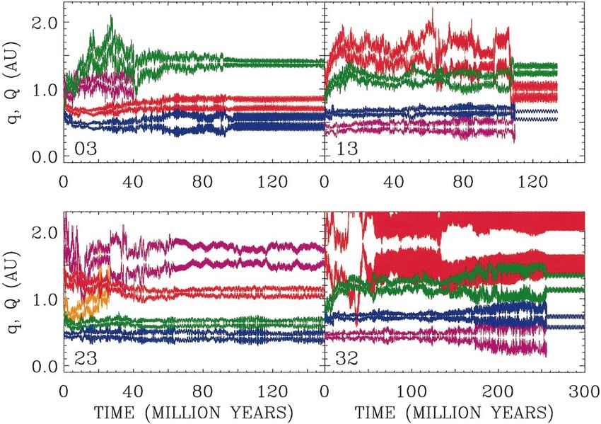
3.1. Sample Evolutions
Jupiter and Saturn were included in each integration from the
beginning. The giant planets started with their current orbits and Figures 1–4 show the evolution of four of the simulations,
masses, and interacted fully with the embryos and planetesimals. one from each batch. Each symbol in the figures shows the semi-
In addition, the initial orbits of Jupiter and Saturn were rotated major axis, a, and eccentricity, e, of an embryo, where the radius
so that the disk of embryos lay in the invariable plane of the of the symbol is proportional to the radius of the embryo. Note
Jupiter–Saturn system. that the values of e and a are the instantaneous values. The
Collisions between objects were assumed to be totally inelas- embryos’ eccentricities generally undergo large oscillations on
tic, so that each collision conserved mass and linear momentum, timescales of 104 –106 years (see Paper I).
and produced a single new body. The new object retained any Figure 1 shows the evolution of simulation 03, which began
excess angular momentum resulting from an oblique impact as with 153 equal mass embryos with eccentricities 0 < e < 0.1
spin angular momentum. In principle, this allows us to calculate and inclinations 0 < i < 5◦ . These values of e and i are quite
the spin rate and obliquity of any object that has accreted another large, so gravitational focusing during close encounters was
body. Collisions were determined by assuming that the embryos weak. As a result, the collision rate was low, even at the be-
are spherical, with radii corresponding to a material density of ginning of the integration. For example, only three collisions
3 g cm−3 . occurred during the first 100,000 years of the integration. In
The integrations used a new hybrid symplectic integrator al- simulation 01, in which e and i were initially smaller by a factor
gorithm (Chambers 1999) and the Mercury integrator package of ten, 24 collisions occurred in the same amount of time.
(Chambers and Migliorini 1997). The integration algorithm is a In simulation 03, the orbits became more dynamically excited
substantial improvement over the combination of symplectic and with time. Near the outer edge of the disk, e increased rapidly
nonsymplectic integrators used in Paper I. The typical energy er- as a result of strong secular perturbations from the giant plan-
ror at the end of one of these integrations (excluding energy loss ets, which peak at the ν6 resonance at 2.1 AU. Objects in the ν6
because of collisions) was about 1 part in 104 . The hybrid inte- resonance experience large, chaotic oscillations in e. These os-
grator parameters are a stepsize of 7 days, and a Bulirsch–Stoer cillations are driven by the coincidence of the rate of precession
tolerance of 10−11 . of the orbit’s longitude of perihelion with an eigenfrequency
In order to avoid excessive integration errors (which rise of the planetary system (which roughly corresponds to the pre-
rapidly with decreasing heliocentric distance r for a fixed- cession frequency of Saturn’s longitude of perihelion). As the
timestep integrator) bodies were assumed to collide with the simulation continued, this excitation propagated to other parts
Sun if their heliocentric distance fell below 0.1 AU. It might be of the disk, as embryos with large e were scattered to smaller
thought that this approximation would artificially bias the results a via close encounters. Some of the embryos were excited to
of the integrations by prematurely removing material on eccen- sufficiently large values of e that they fell into the Sun. In sim-
tric orbits or orbits with small semi-major axes. In practice, these ulation 03, about 25% of the initial mass was lost, almost all
effects turned out to be minor. For example, in simulations 01 of it colliding with the Sun. The corresponding figures for the
and 21, 65 objects were removed with r < 0.1 AU. Of these, 55 other simulations are comparable, although somewhat lower for
had a > 1.8 AU just prior to their removal. These objects were the simulations with initially bimodal mass distributions. The
in, or close to, the asteroid belt, clustered around the ν6 and 3 : 1 mean mass losses for simulations 01–14 and 21–34 were 27%
mean-motion resonances. Such objects are likely to have short and 22%, respectively.208 J. E. CHAMBERS FIG. 1. Evolution of the semi-major axes and eccentricities of embryos from simulation 03. The symbol radius is proportional to the radius of an embryo. In simulation 03, accretion occurred most rapidly in the inner the inner part of the disk had been accreted by two objects, part of the disk, and the largest objects in this region grew to the larger of which had a mass similar to Earth with an orbit ∼0.2M⊕ within a few million years. The accretion rate then similar to Venus. A third large object with a mass of about 0.5M⊕ slowed considerably. By ∼60 million years, all the material in lay further from the Sun with an orbit similar to that of Mars. FIG. 2. Evolution of the semi-major axes and eccentricities of embryos from simulation 13. The symbol radius is proportional to the radius of an embryo.
MAKING MORE TERRESTRIAL PLANETS                                                                  209

  FIG. 3. Evolution of the semi-major axes and eccentricities of embryos from simulation 23. The symbol radius is proportional to the radius of an embryo.

However, this outer region still contained about 10 other bodies,              bodies remaining. The orbits of these large bodies experienced
mainly embryos which had undergone no accretion since the                      only minor changes from 60 million years onward.
start of the simulation. Over the remainder of the integration,                   Figure 2 shows the evolution of simulation 13, which began
these objects were accreted by the larger bodies or fell into                  with 158 embryos with initial masses that increased rapidly with
the Sun in roughly equal numbers, leaving only the three large                 distance from the Sun up to a maximum at a = 0.7 AU, and

  FIG. 4. Evolution of the semi-major axes and eccentricities of embryos from simulation 32. The symbol radius is proportional to the radius of an embryo.
210                                                           J. E. CHAMBERS

then decreased with distance after that. The early stages of the        no accretion. Subsequently, two of the embryos collided, the
evolution were similar to that in Fig. 1. Accretion was most rapid      residual planetesimals were swept up or fell into the Sun, and a
in the inner part of the disk, and strong orbital excitation occurred   system of four planets formed, with characteristics quite similar
near a = 2 AU, which gradually propagated to smaller a. The             to the terrestrial planets. This system proved to be more stable
early accretion rate was also similar to simulation 03. However,        than that of Fig. 2 at 100 Ma, and no further collisions took place.
one object grew faster than the others, and by 10 million years         In this simulation, the structure of the final system of planets was
a “proto-Venus” of about half an Earth mass had formed at a ∼           determined at an early stage—most of the final characteristics
0.6 AU. This planet subsequently grew more slowly, while a              were apparent at 30 million years, and accretion was almost
second larger body accreted at a ∼ 1.1 AU.                              complete by 60 million years.
   By 30 million years, 63% of the original mass was contained in          Figure 4 shows simulation 32, which began with 14 large
four large objects, and these had orbits and masses quite similar       embryos and 140 smaller planetesimals. The masses of both the
to the terrestrial planets. The remaining mass existed in about 40      embryos and the planetesimals were a function of semi-major
smaller planetary embryos, most having a > 1 AU. The four large         axis in a way analogous to the objects in simulation 13 (see
bodies swept up or scattered all the other embryos by 100 million       Fig. 2). However, at any point in the disk the embryos were
years, and formed what appeared to be a stable system. How-             10 times as massive as the planetesimals. In this integration,
ever, the outer two bodies (“Earth” and “Mars”) were too close          the initial values of e and i were low, leading to quite rapid
together—their orbital eccentricities meant that their orbits al-       collisional evolution at first (eight collisions occurred in the first
most crossed one another. Eventually they had a close encounter         105 years). However, the mean e and i increased rapidly, and
which caused them to swap places. This brought Mars into close          were soon comparable to values for simulations beginning with
proximity with “Venus,” which perturbed Venus’s orbit enough            larger e and i.
to cause it to cross the orbit of “Mercury.” The end result was            Partial equipartition of random orbital energy was apparent
that the inner two planets collided with one another, and the           as in simulation 23. The large embryos typically had smaller e
outer two planets swapped places. The final system contained            and i than the less massive planetesimals. Dynamical excitation
three planets in an unusual configuration: two large bodies and         was also pronounced near the ν6 secular resonance, and both
a smaller one in between.                                               embryos and planetesimals were vulnerable to being lost as a
   Figure 3 shows simulation 23, which began with 154 em-               result (e.g., the embryo at a = 2.3 AU in the 30 million year panel
bryos with a bimodal mass distribution. Half the initial mass           of Fig. 4 is about to be lost).
was contained in 14 large embryos, and half in 140 smaller                 The situation at 30 and 100 million years was broadly similar
“planetesimals.” The wide range of masses meant that partial            to Fig. 3. In each case there were three large planets with a <
equipartition of random orbital energy (“dynamical friction”)           2 AU, and a number of bodies further from the Sun. However,
occurred, and for most of the integration the large embryos had         in the simulation of Fig. 4, the inner two planets lay close to
lower e and i than most of the small planetesimals, as can be           a secular resonance with one another, in which their perihelia
seen in Fig. 3. Early in the integration, the orbital excitation        precessed at the same rate. As the two planets moved in and
of the small planetesimals was larger than that of small bod-           out of this resonance, their eccentricities increased until their
ies in simulations 03 and 13, while the excitation of the large         orbits become crossing, and they collided. Meanwhile, most of
embryos in simulation 23 was comparable to that of the largest          the planetesimals in the outer part of the disk were removed,
bodies in the earlier integrations. This apparently contradictory       leaving one tiny survivor with about half the mass of the Moon,
behavior presumably occurs because the largest bodies in sim-           moving on an apparently stable orbit just inside the asteroid
ulation 23 are somewhat more massive than the largest bod-              belt.
ies in simulations 03 and 13 at early epochs, which partially
offsets the greater dynamical friction in the former case, while
                                                                        3.2. Orbital Excitation
the small bodies are less massive than those in simulations 03
and 13.                                                                    One of the problems identified with the simulations in Paper
   In simulation 23, the mass difference between the embryos            I was that the final planets had large orbital eccentricities and
and planetesimals was large enough that the embryos did almost          inclinations. In Figs. 1–4 is it clear that e becomes large for
all of the accreting. A few planetesimals collided with and ac-         many of the embryos in the new simulations, although dynamical
creted other planetesimals, but never gained enough mass to             friction means that the most massive bodies tend to have more
close the gap with the embryos. At 10 million years, the largest        nearly circular orbits.
embryo had a mass of about 0.6M⊕ and a ∼ 1.3 AU. This object               Figure 5 shows the mass-weighted mean eccentricity, ē, versus
had accreted four other embryos so far, plus a small amount of          time in four of the new simulations. Note the change in the scale
mass in planetesimals. Unlike Figs. 1 and 2, in this simulation a       of the x axis at 1 million years. In simulations 03, 13, and 23,
“protoEarth” formed before a proto-Venus.                               which began with large initial e, the mass-weighted eccentricity
   By 30 million years, only five embryos remained. About 25            rose rapidly during the first few hundred thousand years because
planetesimals were still present, most of which had undergone           of close encounters and secular interactions between embryos.
MAKING MORE TERRESTRIAL PLANETS 211
by
q¡
√ £ ¢ ¤
6jm j aj 1 − 1 − e2j cos i j
Sd = √ . (1)
6jm j aj
The behavior in Fig. 6 is somewhat different than in Fig. 5. Al-
though both ē and Sd are mass weighted, the former depends
mostly on e of the largest bodies whereas the latter is strongly
influenced by e and i of the smaller bodies also. This is because
dynamical friction tends to give low-mass bodies large eccen-
tricities and inclinations, and orbits with large e and i make large
contributions to Sd (it is proportional to e2 + i 2 for small e and
i). This is apparent in the occasional spikes seen in Fig. 6, which
are each due to a single body moving on a highly eccentric or-
bit. These bodies quickly fall into the Sun, at which point Sd is
FIG. 5. Mass-weighted eccentricity versus time for the simulations shown reduced again.
in Figs. 1–4. Note the change in scale of the x-axis at 1 million years. Because single objects can make large contributions to Sd ,
its behavior is less smooth than ē as long as orbital and accre-
In simulation 32, which began with initial values of e between tional evolution is still taking place. This allows us to pinpoint
0 and 0.01, the initial rise was greater, but after 0.5 million the damping effects of individual collisions and “evaporations,”
years, ē had become similar to the other simulations. This time which is difficult using ē. For example, the large drop in Sd at
is comparable to the timescale for planetary embryos to form, 0.8 Myr in simulation 32 is caused when the outermost large
which suggests that embryos probably had e > 0.01 at the end embryo falls into the Sun. Correlating changes in Sd with col-
of the runaway growth stage of accretion. lisions or removal events suggest that the loss of high-e objects
The rate of increase in ē slows dramatically in each simula- when they hit the Sun plays a larger role than collisions between
tion when ē reaches about 0.1. At this stage, the largest embryos embryos in damping the orbital excitation of the whole system.
contain 0.1–0.2 Earth masses, and have escape velocities of However, both processes play a part.
5 to 6 kms−1 . At a = 1 AU, this corresponds to about 20% of When accretion ceases, ē still undergoes large oscillations.
the orbital velocity. After a few close encounters with such bod- Conversely, Sd is generally quite well conserved, except in cases
ies, a typical embryo/planetesimal would have an eccentricity such as simulation 01, in which there is strong coupling between
of up to 0.2. the terrestrial planets and Jupiter and Saturn (in this simulation,
At later times the behavior of ē varies from one simulation to one final planet is in the ν5 secular resonance). Sd usually falls
another, but generally ē rises to a maximum of 0.15–0.2 at 50– significantly when accretion ceases and the last planet-crossing
100 million years, and then declines slightly. This decline has
two causes. First, collisions between embryos on eccentric orbits
tend to produce a new body moving on a more circular orbit.
Second, embryos with very high eccentricities are ultimately
removed by collisions with the Sun or ejection from the Solar
System. This “dynamical evaporation” is somewhat analogous
to cooling of a liquid by escape of the most energetic molecules
from its surface.
In the late stages of simulation 32, a deviation from this
trend is apparent. In this integration, ē increased after about
150 million years. This was primarily due to a near secular
resonance between two of the largest embryos. These objects
ultimately collided, reducing ē, but leaving a system that was
still somewhat more excited than average.
Another way to assess the degree of orbital excitation is to use
the angular momentum deficit (Laskar 1997). This measures the
difference between an orbit’s z-component of angular momen-
tum, and that for an orbit with the same semi-major axis having FIG. 6. Normalized angular momentum deficit versus time for the simu-
zero e and i. Figure 6 shows the normalized angular momentum lations shown in Figs. 1–4. Note the change of scale of the x-axis at 1 million
deficit (Sd ) for the simulations shown in Fig. 5, where Sd is given years.212 J. E. CHAMBERS
body is removed. At this point, Sd generally has a value similar
to that during the first million years of the integration. However,
ē usually undergoes a much smaller change upon completion of
accretion. This suggests that the time-averaged eccentricities of
the largest bodies (which dominate the contributions to ē) do not
change significantly once these bodies have formed.
3.3. Evolution of Earth Analogues
In most of the 16 simulations, it is possible to identify ob-
jects at the end of the integration which are reasonable ana-
logues of Earth and Venus in terms of mass and semi-major
axis. (This is usually not true for Mercury and Mars.) We can
use these analogues to gauge possible dynamical and accre-
tional histories for Earth and Venus. In systems containing two
final planets, the inner object “Venus” and the outer object
“Earth” are designated. When N = 4, the second and third plan-
ets were chosen to be Venus and Earth. For cases with N = 3, the FIG. 8. Obliquity versus time for Earth analogues in the simulations shown
choice is somewhat subjective; in general, the inner and outer in Figs. 1–4.
of the two largest planets are chosen to be Venus and Earth,
respectively.
Figure 7 shows the mass of Earth analogues versus time in 4 second phase is characterized by accretion of residual smaller
simulations. In simulations 01–14, objects destined to become bodies, mostly from the outer part of the disk. In a few cases,
Earth analogues usually undergo rapid accretion during the first however, (e.g., simulation 03) the latter phase is absent.
few million years, typically reaching about 20% of their final The median times required for Earth analogues to reach 50%
mass by this time. The accretion rate then slows down. In simu- and 90% of their final mass are 20 and 54 Myr, respectively,
lations 21–34, which began with some large embryos, this phase for the 16 simulations. The median times are similar for the
of accretion is less pronounced. simulations using uniform initial masses and those starting with
At later times, Earth analogues typically go through two more bimodal mass distributions (22, 19 Myr for 50% final mass,
growth phases, with mass growing approximately linearly with and 53, 56 Myr for 90%, respectively) despite the larger initial
time in each phase. This is clearly apparent in simulation 13 in masses of embryos in the bimodal mass cases.
Fig. 7, where there is a rapid rise in mass until about 30 million Most of the Earth analogues experienced giant impacts during
years, followed by slower accretion at later times. The first of their formation. For example, the Earth analogue in simulation
these latter phases appears to be associated with the formation of 03 was hit by another body of almost equal mass at about 40 mil-
a few large protoplanets in the inner parts of the disk, while the lion years, and this impact was essentially the last accretion
event. In other cases, such as the Earth analogue in simulation
13, the largest impactor contributed only about 10% of the final
mass. This diversity illustrates the stochastic nature of accretion
in these simulations. However, the range of behaviors is consis-
tent with the finding of Agnor et al. (1999) that the Earth could
have been hit by an impactor with mass greater than that of Mars,
50–100 million years after the formation of the Solar System,
which led to the formation of the Moon.
The most massive impactor to hit the Earth analogues in each
of the simulations has a median mass of 0.22M⊕ . For these
collisions, the impactor has a median mass of 0.67 times that
of the target. In other words, most Earth analogues were hit by
another body of comparable size at some point in their accretion.
Figure 8 shows the obliquity evolution of the 16 Earth ana-
logues. The high frequency oscillations in the figure are caused
by small variations in the orbital inclinations. The abrupt jumps
are due to collisions with other bodies. These collisions are usu-
ally oblique, so they reorient the spin axis of the body. In some
FIG. 7. Mass versus time for Earth analogues in the simulations shown in cases, this can cause very large changes in the spin orientation.
Figs. 1–4. For example, the Earth analogue in simulation 03 changed fromMAKING MORE TERRESTRIAL PLANETS 213
However, in another quarter of the simulations, e is excited in
the final stages of accretion. This is true in simulation 32, in
which two of the embryos enter a near secular resonance with
one another, which also excites the eccentricities of other bod-
ies in the system. In the remaining 50% of the simulations (e.g.,
simulations 13 and 23 in Fig. 9), the eccentricity of Earth ana-
logues is established early in the integration. In these cases there
is no substantial late-stage excitation or damping in e.
The evolution of Venus analogues is similar to that of Earth
analogues. At early times, the former grew slightly faster than
the latter, reaching 50% of their final mass in a median time of
15 Myr. At later times, the accretion slowed down, and the Venus
analogues reached 90% of their final mass in a median time of
62 Myr. There is a considerable spread in this later time. In one
extreme case (Simulation 32), “Venus” reached 90% of its final
mass 255 Myr after the start of the integration. Conversely, in
FIG. 9. Eccentricity versus time for Earth analogues in the simulations
some simulations Venus was 90% complete after 30–40 Myr.
shown in Figs. 1–4. There is a weak correlation between the 50% formation times
of Earth and Venus analogues, and also for the 90% formation
times. However, the 50% and 90% formation times for the same
planet appear to be uncorrelated. Hence, the Earth and Venus
a prograde rotation with obliquity of about 70◦ to a retrograde
analogues tended to grow at similar rates to one another, but
rotation with an obliquity of about 160◦ in a single impact at
the early accretion rate was not a good indicator of the later
about 30 million years.
accretion rate.
In most of the simulations, the approximate final obliquity
was determined during the first 50 million years or so, since this
3.4. Final Systems
was when the Earth analogues experienced most giant impacts.
However, in three of simulations 31–34, the Earth analogues Figure 10 shows the final configurations of the 16 simula-
experienced substantial spin axis reorientations at much later tions. Each row of symbols in the figure shows the results of
times. An extreme example is simulation 32, which was trans- one simulation, with symbols representing planets. The radius
formed from a prograde rotator with obliquity comparable to of a symbol is proportional to the radius of the planet. The hor-
Earth, to a retrograde rotator spinning almost on its side. This izontal lines through each symbol indicate the perihelion and
transition was caused by two relatively modest impacts, with aphelion distances of the planet’s orbit, and the arrows show the
bodies each about 10% of the final mass of the planet, occurring
later than 150 Myr.
Figure 9 shows the eccentricity evolution for the Earth ana-
logues of Figs. 7 and 8. The high-frequency oscillations in e with
amplitude ∼0.1 are caused by secular perturbations by neigh-
boring planetary embryos and the giant planets. This is similar
to the behavior found in Paper I. These secular oscillations are
large enough that changes in e caused by impacts do not stand
out. A few of the features in Fig. 9 are correlated with changes in
the mass-weighted mean eccentricity, ē, and normalized angular
momentum deficit seen in Fig. 5 and 6. For example, this is true
for the early excitation and subsequent damping in simulation
03, and the late excitation in simulation 32. However, the e of the
Earth analogues does not always follow the system as a whole.
For example, the eccentricity of the Earth-like planet in simu-
lation 23 undergoes oscillations of roughly constant amplitude
despite large changes in ē and Sd .
For the 16 simulations presented here, there is no overall ten-
FIG. 10. Final states of the 16 simulations, where “SS” refers to the inner
dency for e of Earth analogues to increase or decrease in the late
planets of the Solar System, and “01” refers to simulation 01, etc. Each circle
stages of the integrations. In roughly one quarter of the simula- represents a planet with radius proportional to the radius of the symbol. Hori-
tions, e decreases in the late stages of accretion, usually because zontal lines indicates perihelion and aphelion distances, and arrows indicate the
of changes in the secular perturbations by other large bodies. orientations of the planets’ spin axes.214 J. E. CHAMBERS orientation of the planet’s spin axis with respect to its orbital plane (upward-pointing arrows imply obliquities < 90◦ , while down arrows imply obliquities > 90◦ .) Systems with three or four terrestrial planets are common, while in two cases only two planets formed. The simulations presented in this paper typically produced more final planets than the simulations of Paper I, which often ended with only two planets. The final planets in the new simulations have widely spaced orbits when measured in Hill radii, and moderate eccen- tricities and inclinations. The obliquities ² are such that cos ² is distributed approximately at random. Simulations 21–34, which began with bimodal mass distribu- tions, tended to produce more planets (3.5 ± 0.5) than simula- tions 01–14 (2.9 ± 0.6), which began with more uniform mass distributions. Within each set of integrations the results are quite similar in terms of the number of planets, their masses, and semi- major axes. This is in contrast to Paper I, where the results varied greatly from one simulation to the next, even when the initial conditions were similar. Simulations that began with small val- ues of e and i show some tendency to end with more planets (3.4 on average) compared to integrations with large initial e and i (2.9 on average). Figure 11 shows the distribution of masses, m, as a function of semi-major axis for all the final planets in the simulations. The figure also shows the results of Model B from Paper I for comparison. (Of the three models presented in Paper I, Model B had initial conditions that most closely resemble those used in this paper.) The square symbols in each figure represent the terrestrial planets of the Solar System. The planetary systems de- scribed in Paper I had an m–a distribution quite different from FIG. 11. Mass versus semi-major axis for planets produced by the simula- the terrestrial planets. In those simulations, the planetary masses tions reported here and those of Model B from Paper I. tended to decrease with distance from the Sun, rather than in- creasing at first, peaking in the middle and then decreasing, as they do in the Solar System. The simulations described in this paper have an m–a distri- during the integration. This provides some encouragement that bution that resembles that of the terrestrial planets. The most the small mass of the real Mars can be explained, but note that massive objects have 0.6 < a < 1.2 AU, and objects outside this these low-mass objects all had orbits further from the Sun than range tend to be smaller. The least massive planets usually have Mars does. a < 0.5 AU or a > 1.5 AU. However, planets with orbits simi- The largest planet in each system has a mass similar to Earth. lar to Mars and Mercury generally are more massive than these This reflects the fact that the simulations began with total mass planets. Wetherill (1992, 1996) obtained rather similar results in ∼2.5M⊕ , and typically ended with two or three large planets. simulations using the Öpik–Arnold method, although Wetherill All of the final planets have 0.3 < a < 2.0 AU, correspond- (1992) also found many cases of low-mass planets in the region ing to the initial extent of the disk of embryos. Several bod- occupied by Earth and Venus in the Solar System. ies in each simulation entered the inner asteroid belt, but they The analogues of Mercury are large despite the fact that the were subsequently either lost or returned to the terrestrial-planet initial surface density profile was chosen to keep the amount region. of mass in the innermost part of the disk quite low. Simula- Figure 12 shows the eccentricity versus mass distribution for tions 11–14 and 31–34, in which the embryos decreased in size the final planets in the systems described here, and those of with distance from the Sun, often produced Mars analogues Paper I. The eccentricities, e, have been time-averaged in each that are more massive than this planet, just like the other sim- case. The values of e are generally somewhat smaller in the new ulations presented here and the simulations in Paper I. Inter- integrations than in the old, with the lowest values comparable to estingly, three of the new simulations ended with very small the time-averaged values for Earth and Venus. The median value objects on orbits with 1.5 < a < 2.0 AU. These bodies are all in the simulations, e = 0.08, is somewhat larger than for Earth approximately lunar-mass embryos that underwent no collisions and Venus, but comparable to the time-averaged eccentricity of
MAKING MORE TERRESTRIAL PLANETS 215
four of the zones. The different composition of Earth and Venus
analogues on the one hand and Mars analogues on the other is
consistent with the fact that several elemental and isotopic dif-
ferences are observed between these planets (see discussion in
Taylor (1999)).
The degree of radial mixing is quantified and discussed further
in Section 4.
4. DISCUSSION
Here we return to the questions posed in the introduction:
Why do the results of earlier computer simulations differ from
the terrestrial planets in the Solar System; and are the differences
the result of shortcomings in the computer models, or do they
indicate that our planetary system is special?
To address these questions, we need some criteria to quantify
similarities and differences between systems of terrestrial plan-
ets. We can start by identifying some dynamical characteristics
of the inner planets in the Solar System:
• There are four terrestrial planets.
• The largest (Earth) contains about half of the total mass.
• The planets have orbits that are widely spaced (when mea-
sured in Hill radii).
• Their orbits are almost circular.
• Their orbits are almost coplanar.
• Their spin axes are almost perpendicular to their orbital
planes.
• Most of the mass is concentrated in a narrow range of he-
liocentric distance occupied by Venus and Earth.
FIG. 12. Eccentricity versus mass for planets produced by the simulations
reported here and those of Model B from Paper I.
To quantify these characteristics for any system of terrestrial
planets, using the following statistics is suggested. Each is a
dimensionless quantity, which can also be applied to satellite
Mars. In contrast to the terrestrial planets, there is apparently no systems, systems of giant planets, and so forth.
correlation between e and m in Fig. 12.
Figure 13 shows the composition of the final planets in terms • N , the number of bodies.
of their constituent embryos. The embryos are color-coded in • The fraction of the total mass in the largest object, Sm . This
terms of their initial semi-major axes, with four different shades statistic is unlikely to be completely independent of N , although
of grey implying zones bounded by 0.7, 1.1, and 1.5 AU. The the correlation between the two is not as strong as one might
radius of each pie-chart symbol is proportional to the radius of expect. For example, Saturn’s satellite system contains many
the planet. moons, but 96% of the total mass is contained in one object.
The figure indicates that a considerable amount of radial mix- • An orbital spacing statistic
ing of material occurred during the simulations. However, the µ ¶µ 
final planets have a composition gradient which preserves some 6 amax − amin 3m cen 1/4
Ss = , (2)
memory of the initial distribution of embryos (this is similar to N − 1 amax + amin 2m̄
the result found by Wetherill (1994)). The planets are predom-
inantly composed of embryos from one or two zones closest where m̄ is the mean mass of the planets/satellites, m cen is the
to their final semi-major axis. This is especially true of small mass of the central body (e.g., the Sun), and amax and amin
planets that are closest to or furthest from the Sun (possible ana- are maximum and minimum semi-major axes. This statistic
logues of Mercury and Mars). In particular, the “Mercuries” tend is somewhat similar to the mean spacing in Hill radii. How-
to contain material that mostly comes from the innermost zone, ever, we can use the observation of Chambers et al. (1996)
while “Marses” are mostly made of embryos from the outer that the stability of a planetary system is proportional to the
two zones. Analogues of Earth and Venus, on the other hand, orbital spacing measured using a quantity, R1/4 , that varies as
usually contain significant amounts of material from three or m 1/4 rather than the Hill radius, which varies as m 1/3 . The216 J. E. CHAMBERS
FIG. 13. Composition of the final planets in eight simulations as a function of the initial location of the embryos that comprise each object. Symbol size is
proportional to the radius of each planet.
normalizing factor of 6 is chosen to make Ss similar to the mean • A mass-concentration statistic
spacing of the terrestrial planets in Hill radii. µ 
• The normalized angular momentum deficit, Sd , defined in 6m j
Sc = max , (4)
Eq. 1. This is chosen rather than the mass-weighted e or i since 6m j [log10 (a/a j )]2
Sd generally undergoes smaller changes over time.
• An obliquity statistic where m j and a j are the mass and semi-major axis of each planet,
µX ¶Á and Sc is given by the maximum value of the function in brackets
as a function of a. This statistic measures the degree to which
So = |cos ² j | N, (3)
mass is concentrated in one part of the planetary system (e.g.,
in the narrow range of semi-major axes spanned by Earth and
where ² j is the obliquity of planet j. This statistic measures Venus in the case of the terrestrial planets). The logarithm of a is
the degree to which the spin axes of the planets/satellites are used since there is some indication that planetary spacings in the
perpendicular to their orbital planes. Randomly orientated spin Solar System increase in proportion to heliocentric distance (the
axes would make So = 0.5 on average. essence of the Titus–Bode law). To help understand the meaningMAKING MORE TERRESTRIAL PLANETS 217
so it is not possible to calculate So in these cases. Finally, the
relevant statistics for the large members of the satellites systems
of Jupiter, Saturn, and Uranus are given. While it is currently un-
clear how these systems formed, they obey the same dynamical
laws as systems of terrestrial planets. As a result, comparisons
between the two should help to determine whether planetary
orbits are primarily determined by processes occurring during
formation, or dynamical effects subsequently.
Figure 15 shows the range of values of these statistics for
the various simulations, and shows the location of the terrestrial
planets within these distributions. Figure 16 indicates the degree
of correlation (if any) between various pairs of statistics.
4.1. Number of Planets, Orbital Spacing, and Radial Mixing
These issues are closely related, so they are considered to-
gether. The number of final planets, N , depends on the range of
their semi-major axes amax –amin , and their orbital spacing, Ss . In
FIG. 14. Examples of the function used in the Sc statistic for four planetary
systems, including the terrestrial planets (lower right). The radius of each planet
TABLE I
is proportional to the radius of the symbol. The Sc statistic is given by the
maximum value of the function. Statistics for Final Planetary Systems
Sim N Sm Ss Sd So Sc Sr
of Sc , Fig. 14 shows some examples of the function in brackets in
Eq. 4. The four panels of the figure show the function for three 01 3 0.600 45.6 0.0502 0.49 38.9 0.406
02 3 0.387 36.0 0.0041 0.39 48.8 0.371
systems containing equal mass planets, and for the terrestrial 03 3 0.544 41.4 0.0102 0.86 45.1 0.420
planets of the Solar System (lower right panel). The semi-major 04 2 0.545 47.2 0.0032 0.19 63.0 0.341
axes of the planets in each system are shown by the circular 11 3 0.412 38.5 0.0061 0.41 40.9 0.383
symbols. In each panel, Sc is given by the maximum value of 12 4 0.393 37.1 0.0043 0.46 47.0 0.390
the curve as a function of a. 13 3 0.455 32.0 0.0045 0.33 41.7 0.337
14 2 0.722 52.1 0.0140 0.52 60.3 0.453
• A radial-mixing statistic
·X ¸Á X 21 4 0.335 31.3 0.0045 0.31 37.3 0.275
m i |ainit,i − afin,i | 22 4 0.326 33.7 0.0102 0.42 35.0 0.262
Sr = mi , (5) 23 4 0.493 36.4 0.0048 0.73 34.8 0.263
afin,i
24 3 0.471 44.7 0.0052 0.46 32.4 0.290
31 4 0.456 35.4 0.0036 0.69 36.8 0.271
where ainit and m are the initial semi-major axis and mass of 32 3 0.616 42.6 0.0093 0.40 53.8 0.271
each embryo that becomes incorporated into a final planet, and 33 3 0.715 44.6 0.0060 0.33 63.8 0.341
afin is the semi-major axis of that planet. 34 3 0.616 44.9 0.0107 0.64 45.2 0.208
This statistic sums the radial migrations of each embryo that
contributes toward a final planet, weighted according to the em- Paper I median 2.4 0.694 53.8 0.0228 — 39.0
C 1998 median 3.0 0.511 42.4 0.0103 — 45.1
bryo’s mass. The value of Sr cannot be compared directly with 01–14 median 2.9 0.500 40.0 0.0053 0.44 46.1 0.384
the terrestrial planets of the Solar System, since the source re- 21–34 median 3.5 0.482 39.5 0.0056 0.44 37.1 0.273
gions for the material contained in these planets is not known.
However, Sr allows the degree of radial mixing to be compared MVEM 4 0.509 37.7 0.0018 0.96 89.9
between simulations. JSUN 4 0.715 11.6 0.0012 0.73 26.9
Jupiter I-IV 4 0.378 16.5 4e-5 1.00 17.8
Saturn I-VIII 8 0.955 11.4 0.0012 104.6
Table I shows the values of these statistics for the planetary
Uranus I-V 5 0.386 15.6 2e-5 1.00 32.8
systems produced by the 16 simulations described in this paper.
The table includes the statistics for the inner planets of the Solar Note. N is number of final planets, Sm the fraction of mass in the largest
System, and median values for systems produced in Paper I (note object, Ss is the orbital spacing statistic (see text), Sd is the normalized angu-
that the values of N are means rather than medians), and for an- lar momentum deficit, So is the mean value of |cos ²| where ² is the obliquity
of each planet, Sc is the mass concentration statistic, and Sr is a radial mix-
other set of N-body simulations in Chambers (1998; referred to
ing statistic (see text). “Paper I” refers to nine simulations from Model B of
as C98 from now on), which began with 80–120 embryos and Paper I. “C 1998” refers to eight simulations from Chambers (1998). “MVEM”
nonuniform mass distributions. Note the simulations in C98 and refers to the system Mercury, Venus, Earth, and Mars. “JSUN” refers to the
Paper I did not record changes in the spin states of the embryos, system Jupiter, Saturn, Uranus, and Neptune.218 J. E. CHAMBERS
a strong inverse correlation between N and the orbital spacing
Ss in the simulations, whereas one might expect that the typical
spacing would be independent of N . This suggests that the fi-
nal planets retain some memory of the radial extent of the disk
of embryos from which they formed; Wetherill (1994) reached
a similar conclusion. In simulations with few final planets, the
orbits tend to be widely spaced, occupying a greater semi-major
axis range than they would do if their orbital spacing was com-
parable to cases with more final planets.
The orbits of the terrestrial planets are very widely spaced
compared to those of the giant planets or their satellites sys-
tems (see Table I). This is true whether we measure spacing in
terms of the Hill radius, R H , which varies as m 1/3 , or a quantity
Ss that varies as m 1/4 . The giant planets and their satellite sys-
tems may have formed in ways very different than the terrestrial
planets, but each system has obeyed the same laws governing
gravitational interactions since then. For example, Chambers
FIG. 15. Range of values of the statistics for planetary systems produced by et al. (1996) have shown that a system of planets with similar
the simulations described in this paper. The three points on each line indicate the masses, initially moving on circular orbits, is stable for a time
minimum, median (mean for N ) and maximum values for each set of simulations. that depends only on the mean spacing in R1/4 . As a result, the
Also shown are the statistics for simulations using Model B of Paper I (P1),
and the integrations of Chambers 1998 (C98). The diamond symbols show the
very wide spacing of the terrestrial planets compared to other
statistics for the terrestrial planets. systems requires an explanation.
Laskar (1997) has made a stability analysis of the planetary
system which suggests that there is no room to fit extra planets
addition, if we measure orbital spacing in terms of quantities that into the terrestrial region (except possibly interior to Mercury).
depend on mass, such as R H or R1/4 , the final number of planets This is because the eccentricities of the inner planets undergo
can depend upon their masses also. large oscillations on long timescales, which would make the
The maximum semi-major axis a that a planet in the inner orbit of any intermediate planet unstable. In Laskar’s model,
Solar System can have is about 2.0 AU, which is determined by the angular momentum deficit, Sd , of the terrestrial planets is
the location of the ν6 secular resonance. The minimum value essentially a conserved quantity, and exchange of Sd between
of a is less clear. The steep potential gradient close to the Sun the inner planets determines the degree of their possible radial
probably prevented planets forming very much interior to the excursions. In practice, some exchange of Sd with the outer
semi-major axis of the innermost planetary embryos that existed. planets occurs, but this is usually < 50% of the total value for
This distance may have been determined by several factors, such the inner planets over the age of the Solar System; see Fig. 1 of
as the heliocentric distance at which condensible material could Laskar (1997).
exist when plantesimals and embryos were forming; the distance Hence, in Laskar’s model, the Sd of Mercury, Venus, Earth,
at which embryos would have been destroyed by collisional and Mars, immediately after they had accreted, determined that
fragmentation (which depends on the Keplerian velocity and these would be the only terrestrial planets in the Solar System.
hence a); clearing processes associated with the young Sun; However, this argument does not explain why the Solar System
and so forth. Apparently, embryos existed at ∼0.4 AU in order has four terrestrial planets. To see this, imagine that the semi-
to form Mercury, but they may also have existed closer to the major axes of the inner planets were rearranged, placing them
Sun. slightly closer together, and making use of the space interior
The maximum semi-major axis range constrains the maxi- to Mercury and exterior to Mars. In addition, suppose that the
mum value of N , but not the minimum value. Terrestrial planets ∼2M¯ of mass contained in the inner planets was redistributed
do not have to occupy all of the semi-major axis space available so that the planets either had a larger or smaller range of masses
to them. For example, in the Solar System there is a wide gap be- than today. Using some combination of these processes, it seems
tween the orbit of Mars and the ν6 resonance. As Fig. 10 shows, likely that systems of five or even six terrestrial planets could
the outermost terrestrial planet could have formed on a stable exist, with stable orbits, and with the same value of Sd as the
orbit with larger a than Mars. The figure also shows a wide inner planets of the Solar System. Conversely, it is certainly true
variety in the semi-major axis ranges of the planetary systems that fewer than four inner planets could exist, with the same to-
produced in the simulations. For example, compare simulation tal mass and angular momentum deficit as the terrestrial planets.
12 (values of a spanning 1.4 AU) with simulation 14 (a range of So, while the model of Laskar (1997) makes an important con-
0.7 AU). These calculations began with quite similar initial con- tribution to our understanding of the configuration of the inner
ditions, yet ended very differently. Interestingly, there is quite planets, it is clearly not the whole story.You can also read