Fine scale variation in projected climate change presents opportunities for biodiversity conservation in Europe
←
→
Page content transcription
If your browser does not render page correctly, please read the page content below
www.nature.com/scientificreports
OPEN Fine‑scale variation in projected
climate change presents
opportunities for biodiversity
conservation in Europe
Tomáš Hlásny1, Martin Mokroš1, Laura Dobor1, Katarína Merganičová1 & Martin Lukac1,2*
Climate change is a major threat to global biodiversity, although projected changes show remarkable
geographical and temporal variability. Understanding this variability allows for the identification
of regions where the present-day conservation objectives may be at risk or where opportunities for
biodiversity conservation emerge. We use a multi-model ensemble of regional climate models to
identify areas with significantly high and low climate stability persistent throughout the twenty-
first century in Europe. We then confront our predictions with the land coverage of three prominent
biodiversity conservation initiatives at two scales. The continental-scale assessment shows that
areas with the least stable future climate in Europe are likely to occur at low and high latitudes, with
the Iberian Peninsula and the Boreal zones identified as prominent areas of low climatic stability. A
follow-up regional scale investigation shows that robust climatic refugia exist even within the highly
exposed southern and northern macro-regions. About 23–31% of assessed biodiversity conservation
sites in Europe coincide with areas of high future climate stability, we contend that these sites should
be prioritised in the formulation of future conservation priorities as the stability of future climate
is one of the key factors determining their conservation prospects. Although such focus on climate
refugia cannot halt the ongoing biodiversity loss, along with measures such as resilience-based
stewardship, it may improve the effectiveness of biodiversity conservation under climate change.
Rapid climate change induced by human activity is already changing the distribution of a great number of
species1,2. Current commitments under the Paris COP21 agreement are unlikely to keep planetary warming
below 2 °C considered safe, plus several feedback mechanisms and climate tipping points threaten to exacerbate
it further3. Climate change is thus one of the key threats to biodiversity at all levels; from genes to biomes4. On
the one hand, effects of climate change range from local extinctions of species with narrow ecological niches, to
profound ecosystem change at the trailing edge of the shifting climatic e nvelope5. On the other hand, we already
see increased species richness in areas acting as refugia and effects such as the Northern Biodiversity P aradox6.
Recent observations from Europe show a significant decrease in mountain species richness in the Mediterranean
and a concurrent increase in the boreal–temperate z one7. Climatic processes driving these changes include the
emergence of novel climates, rapid displacement of climatic isoclines, or the divergence of temperature and
precipitation vectors8, all resulting in significant shifts of species distribution.
Species extinctions and migration are likely to generate novel communities and thus challenge the contempo-
rary conservation planning f ramework9, which relies on a fixed system of protected areas and conservation goals.
Rapid climate change highlights the need for accommodating transient ecosystem dynamics into conservation
planning9,10, yet practical implementation of climate change adaptation into conservation management is still
rare11. Recent climate-adapted conservation concepts include an evaluation of species vulnerability by empirical
niche models12, use of climatic refugia to shelter species of conservation concern13, or the implementation of
resilience-oriented ecosystem management14. However, the theoretical understanding of these approaches, their
trade-offs, and interactions is not sufficiently advanced to support the formulation of robust and consistent con-
servation policies. A better understanding may stimulate a broader shift in governance structures and improved
coordination between land managers, politicians, and conservation organisations which appears critical to the
implementation of adaptive biodiversity c onservation15.
1
Faculty of Forestry and Wood Sciences, Czech University of Life Sciences Prague, Kamýcká 129, 165 00 Prague,
Czechia. 2School of Agriculture, Policy and Development, University of Reading, Reading RG6 6AR, UK. *email:
m.lukac@reading.ac.uk
Scientific Reports | (2021) 11:17242 | https://doi.org/10.1038/s41598-021-96717-6 1
Vol.:(0123456789)
www.nature.com/scientificreports/
ID Abbreviations Description Units Calculation
1 MWMT Mean warmest month temperature °C MWMT = max(Tmon.mean )
T − 5 ◦ C, T > 5 ◦ C
2 DDa5 Degree-days above 5 °C °C
DDa5 = doy 0 ◦ C, T < 5 ◦C
The length of the longest period of consecutive days with daily
3 FFP Longest frost-free period Days
minimum temperature above 0 °C
4 EQ Ellenberg climatic quotient °C mm−1 EQ = MWMT
× 1000
Pr ann
5 Cont Gorczynski climatic continentality –
Cont = 1.7 × MWMT−MCMT
sinϕ − 20.4
1, Pr < 5mm
DryDay = 0, Pr > 5mm
6 NDP Number of dry periods –
DryPeriod: period of at least 10 consecutive DryDays
numDryPeriods: the number of DryPeriods
7 LLDP Length of the longest dry period Days Number of dry days of the longest DryPeriod
8 T Annual mean temperature °C Average of daily mean temperatures
9 P Annual total precipitation mm Sum of daily precipitations
Table 1. Climate variables used as predictors of future climate stability, all calculated on annual basis (T
temperature, Pr precipitation, MCMT mean coldest month temperature).
In Europe, Key Biodiversity Areas ( KBA16), Natura 2000 habitat n etwork17, and European Primary Forests
(EPF18) represent examples of biodiversity conservation initiatives focused on preserving geographically well-
defined areas of interest. Under climate change, some of these areas and associated conservation goals may be
subject to greater climatic exposure than others. At the same time, conservation opportunities may emerge
elsewhere due to future spatial or temporal variation of climate change effects. Focusing on areas with pre-
dicted stable climate, relative to background climate change, is increasingly recognised as a viable conservation
strategy19–21. These climatic refugia may arice at multiple spatial scales, from small-scale poleward-facing slopes,
sites affected by cold groundwater or deep snow drifts22, to the continental-scale refugia such as the Boreal zone
in Europe6. Descriptions of species migration and persistence in climatic refugia during glacial and interglacial
periods may be applicable to present-day conservation effort19, if future climate can be resolved at an appropriate
scale. Climate models, which have an increasing ability to resolve the fine-scale atmospheric processes relevant
for local and regional resource management and conservation planning, have thus become the central means
for formulating forward-looking adaptation policies23.
We investigate how future climate change may affect present-day nature conservation initiatives in Europe,
by considering spatial coverage and temporal persistence of regions with significantly lower or higher climatic
stability. This information may be vital for the transition from the current static conservation framework to
climate-adapted conservation strategies deemed necessary to avoid the imminent biodiversity b reakdown24. At
continental and regional scales, we confront climatic stability patterns with established biodiversity conservation
initiatives, ranging in size from the Global Biodiversity Hotspots to small patches of primary forests. Representing
the diversity of spatial scales at which atmospheric and biological processes operate25, we (i) evaluate the patterns
of projected climatic stability in Europe at two scales; (ii) indicate some of the existing biodiversity conservation
sites exposed to future high or low risk of climatic stability, and (iii) discuss how the identification of such sites
can inform the formation of a climate-adapted biodiversity conservation strategy for Europe.
Results
Our analysis of future climatic stability is based on projected changes of nine climate variables, selected to proxy
key aspects of terrestrial ecosystem dynamics (Table 1). The cumulative change of all nine climate variables,
termed Aggregate Climate Change (ACC), is used to identify regions of significantly higher or lower climatic sta-
bility (Getis-Ord Gi* p-value < 0.05) across Europe. We carry out this assessment at the continental and regional
scales. While the continental assessment reports the large-scale latitudinal and orographic patterns of climatic
stability (Eq. (1), Fig. S3), the regional assessment explores the residual ACC variation that remains after the
extraction of the large-scale continental trend (Eq. (5), Fig. S3). We aim to identify and interpret climatic features
likely to persist in their location throughout the twenty-first century (i.e. in periods 2021–2040, 2041–2060, and
2061–2100) and are supported by a majority of climate projections considered in this study. Areas of persistently
low ACC are henceforth interpreted as potential climatic refugia and we investigate their overlap with existing
biodiversity conservation initiatives.
Continental‑scale assessment. At this scale, future climate variation in Europe displays a distinct latitu-
dinal pattern. This pattern is robust and consistent across all three periods and both RCP scenarios considered
(Fig. 1). Temporal stability of identified climatic features and inter-model agreement were poorer at higher lati-
tudes than in the rest of Europe (Figs. S1, S2). Continental-scale Central Zone (CZ) with the most stable future
climate is located across the centre of Europe (ca 45°–55° N) and covers most of the Atlantic, Continental, and
Steppic biogeographical zones (Fig. S1). The Northern and the Southern Zones located at high and low latitudes
of Europe are characterised by future climate with significantly lower stability (NZ and SZ, respectively). The SZ
extends over the Mediterranean and Anatolia, while the NZ takes in the Boreal and the Arctic regions.
Scientific Reports | (2021) 11:17242 | https://doi.org/10.1038/s41598-021-96717-6 2
Vol:.(1234567890)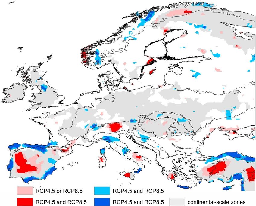
www.nature.com/scientificreports/

                                  Figure 1.  Continental-scale zones with significantly higher (blue) and lower (red) future climate stability,
                                  relative to background climate change. Coloured zones are likely to persist in all periods considered here
                                  (2041–2060, 2061–2080, and 2081–2100). Shading represents zones identified by either (light shade) or both
                                  (dark shade) RCP4.5 and RCP8.5 scenarios. Numbers show geographical sub-zones described in Table 1 and
                                  Fig. 2. Maps were created in R v. 4.0.4. (R Core Team, Vienna, Austria) and ArcGIS Desktop v. 10.7 (Esri,
                                  California, USA). The final layout was created in ArcGIS Desktop v. 10.7 (Esri, California, USA) and CorelDraw
                                  v. 20.1.0.707 (2018 Corel Corp.).

                                     The combinations of predicted changes in individual climate variables are specific to each of the major zones
                                  and their subzones (Fig. 2, Table S3). For example, the magnitude of ACC in the CZ is around 51–55% of the
                                  maximum permissible change (i.e. change that would occur if the largest change in all underlying climate vari-
                                  ables predicted across Europe were to occur in the same pixel), whereas that predicted for the NZ or the SZ is
                                  between 65 and 75% (Table 2).
                                     Looking at zones of low climatic stability predicted under RCP 8.5, the most distinctive features of the NZ are
                                  increased precipitation (+ 143 mm, 25%), shorter dry periods (− 9 days), longer frost-free periods (+ 80 days),
                                  and a strong temperature increase (+ 5.9 °C). The most striking climate features driving low climate stability in
                                  the SZ are the severe decrease of precipitation (− 153 mm, − 24%), and accompanying increases of the Ellenberg
                                  climate quotient (+ 21 to 23 mm °C−1) and of growing degree-days (+ 1484 to 1562 dd). Projected change in cli-
                                  matic continentality is another feature that underlies the difference between NZ and SZ. The patterns of change
                                  projected under RCP4.5 are similar to RCP8.5, however predicted changes are less pronounced (Fig. 2, Table S3).

                                  Regional‑scale assessment. Regional-scale variation of ACC is revealed by the subtraction of the con-
                                  tinental-scale change and creates a mosaic of areas with significantly low and high climatic stability distributed
                                  all over Europe (Fig. 3). In contrast to the continental scale, the regional climatic features show poorer temporal
                                  stability and inter-RCP agreement (Fig. S2). However, a number of areas characterised by residual ACC sig-
                                  nificantly different from background persists throughout the twenty-first century under the most conservative
                                  assessment (areas identified by four out of five RMS in each RCP, Table S3).
                                      At this scale, the most distinct areas with low climatic stability are located within the continental SZ (Fig. 1),
                                  emphasising the high regional variability of ACC in the Mediterranean. Looking at the central band identified
                                  as stable at the continental scale (CZ, Fig. 1), Eastern Alps and parts of Norway now show up as areas with
                                  regionally low climate stability. Crucially, some areas with low and high climatic stability are not too distant,
                                  e.g. seashore to inland transitions or elevation differences in mountain ranges, generating a pattern of climatic
                                  exposure potentially complicating future conservation effort.

Scientific Reports |   (2021) 11:17242 |               https://doi.org/10.1038/s41598-021-96717-6                                                     3

                                                                                                                                                 Vol.:(0123456789)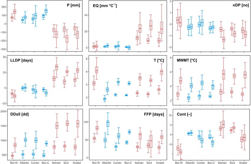
www.nature.com/scientificreports/
Figure 2. Predicted change in nine climatic variables in the geographical subzones predicted to have high
or low future climatic stability (numbering of zones corresponds with Fig. 1). Boxplot pairs show projected
changes driven by RCP4.5 (left) and RCP8.5 (right) and indicate their variation within each subzone. Colours
indicate subzones with predicted low (red) and high (blue) climate stability. Variable acronyms: P annual total
precipitation [mm], EQ Ellenberg climatic quotient [°C m m−1], nDP number of dry periods [no], LLDP length
of the longest dry period [days], T annual mean temperature [°C], MWMT mean warmest month temperature
[°C], DDa5 degree-days above 5 °C [dd], FFP longest frost-free period [days], Cont Gorczynski climatic
continentality [–]. The graphs were created in R v. 4.0.4.26.
Code Zone Sub-zone ACC%—RCP4.5 ACC%—RCP8.5 Climate stability
1 NZ Boreal 74.3 64.4 Low
2 Atlantic 55.3 51.4 High
3 CZ Contin 53.2 50.9 High
4 Boreal 61.6 53.5 High
5 Iberian 75.0 75.7 Low
6 Sicilian 70.4 70.8 Low
SZ
7 Anatolian 74.0 72.5 Low
8 Step 60.4 – High
Table 2. Relative aggregate climate change (ACC%) in zones of low and high climatic stability as indicated
by continental-scale assessment. The position of zones and sub-zones and the numerical codes correspond to
Fig. 1. NZ Northern Zone, CZ Central Zone, SZ Southern Zone.
Spatial coincidence of conservation priorities and climate stability areas. To consider the long-
term implications of contrasting climatic stability for nature conservation efforts in Europe, we confront the
coverage of prominent biodiversity conservation networks (Fig. 4, Supplementary Fig. S4) with continental and
regional areas of contrasting climate stability persisting between 2040 and 2100.
Our predictions indicate a high probability of a significant continental-scale northern zone of low climatic
stability covering northern Finland and Karelia (Fig. 1). This trend represents a clear threat to the Natura 2000
and KBA areas present in northern Finland. Currently, only one forest has been identified as EPF in the country,
not allowing us to draw conclusions concerning this network. Looking at the predictions analysed at the regional
Scientific Reports | (2021) 11:17242 | https://doi.org/10.1038/s41598-021-96717-6 4
Vol:.(1234567890)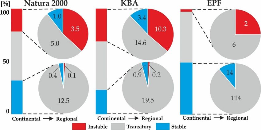
www.nature.com/scientificreports/
Figure 3. Regionally relevant zones of low (red) and high (blue) future climate stability in Europe, relative to
background climate change. Coloured zones are likely to persist in all periods considered here (2041–2060,
2061–2080, and 2081–2100). Shading represents zones identified by either (light shade) or both (dark shade)
RCP4.5 and RCP8.5 scenarios. Grey areas indicate continental scale for reference (Fig. 1). Maps were created in
R v. 4.0.4.26 and ArcGIS Desktop v. 10.7 (Esri, California, USA). The final layout was created in ArcGIS Desktop
v. 10.7 (Esri, California, USA) and CorelDraw v. 20.1.0.707 (2018 Corel Corp.).
scale, it is possible to identify several current biodiversity sites likely to fall under more stable future climate
conditions than others (Fig. 4). Specifically, our data indicate that Natura 2000 and KBA sites in central Norway
are significantly less exposed than those straddling the border between Norway and Finland.
Our continental-scale assessment shows that the central zone area of Europe stretching from the British Isles
in the west to the Ukrainian steppe in the east is likely to experience significantly weaker climate change than the
rest of the continent (Fig. 2, Table S3). Regional-scale assessment however shows that the greatest share of the
KBA extent under future low stability climate is in the Pannonian, Steppic, Mediterranean and Anatolian zones
(see Fig. S3 for the position of biogeographical zones). The above-average share of the KBA sites in zones with
high climatic stability is in the Alpine North and Atlantic zones, the Arctic, and the Black Sea zones; in the latter
two zones, however, the total area of the KBA sites is only minor (Fig. 5). The Alpine zone includes 119 out of
257 primary forests currently described in Europe, a continental-scale assessment shows that 100% of these are
in an area with predicted low climate stability. However, the finer-scale modelling shows that only 11% of these
sites are threatened by significantly low stability climate.
The southern zone shows the lowest climatic stability in Europe at the continental scale and largely overlaps
with Europe’s prominent global biodiversity hotspot—the Mediterranean Basin. It also covers all European parts
of the Irano-Anatolian and the Caucasus zones (Fig. S6). The SZ thus affects all global biodiversity sub-hotpots
embedded within the Mediterranean Basin: the Rif-Betique range, Maritime and Ligurian Alps, Tyrrhenian
Islands, southern and central Greece, Crete, southern Turkey and C yprus27. Our model prediction at this scale
thus delivers a very bleak message for biodiversity conservation sites in and around the Mediterranean.
Discussion
Rapid and accelerating biodiversity loss due to climate change and other anthropogenic factors28,29 has high-
lighted the vulnerability of the current conservation effort, which historically did not take account of projected
climate change9. Some areas of high biodiversity value in Europe are under increasing t hreat30, the update of
their conservation strategies requires location-specific information on future viability31. Whilst the conservation
Scientific Reports | (2021) 11:17242 | https://doi.org/10.1038/s41598-021-96717-6 5
Vol.:(0123456789)www.nature.com/scientificreports/
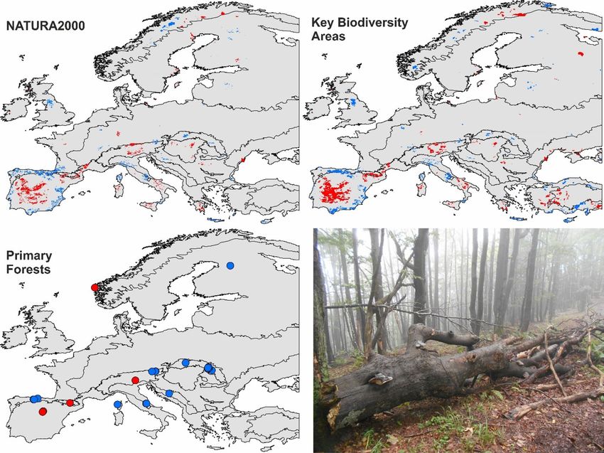
Figure 4. Geographical coverage of existing biodiversity conservation within areas of low (blue) or high (red)
regional-scale climate stability persisting throughout the twenty-first century. Maps were created in ArcGIS
Desktop v. 10.7 (Esri, California, USA). The final layout was created in ArcGIS Desktop v. 10.7 (Esri, California,
USA) and CorelDraw v. 20.1.0.707 (2018 Corel Corp.). The photo illustrates a primary beech forest in the
Western Carpathians, Kremnické Mts., Slovakia. Credit: Merganičová, K.
Figure 5. The proportion of Natura 2000, Key Biodiversity Areas, and European primary forests present in
areas identified as zones of low and high climatic stability, relative to background climate change. Modelling
was carried out at a continental (bars) and regional (pie chats) scales. Values in pie charts indicate areas of
Natura2000 and KBA sites (mil. of ha), or the number of EPF in each climate stability category. Climatic stability
as predicted under RCP4.5 or RCP8.5 and persisting throughout 2041–2100. Graphs were created in R v. 4.0.4.26.
The final layout was created in CorelDraw v. 20.1.0.707 (2018 Corel Corp.).
Scientific Reports | (2021) 11:17242 | https://doi.org/10.1038/s41598-021-96717-6 6
Vol:.(1234567890)www.nature.com/scientificreports/
of biodiversity and its planning is clearly important at the global scale32,33, most species are composed of local
populations, the survival of which is driven by local climate and environment variation34. Emerging capability
of climate models to resolve small-scale atmospheric processes allows for the identification of refugial features
within the landscape35, offering new opportunities for confronting conservation planning with future climate
stability.
Continental scale. According to our continental-scale predictions for Europe, the most stable climate will
persist in the Atlantic and Temperate zones, whilst the Mediterranean and the Boreal zones may be exposed to
the least stable climate (Fig. 1), confirming existing global or continental climatic a ssessments36,37.
Although the lack of future climatic stability is similar in the northern and southern zones, the underlying
changes in climatic variables are distinctly different and so are the risk factors affecting biodiversity. Increasing
drought incidence at low latitudes (e.g. precipitation decreasing by > 23% and the Ellenberg quotient increasing
by up to 23 mm °C−1; Table 1) can cause many valuable ecosystems to collapse and biodiversity to decline38.
Already, the biodiversity in the Mediterranean is showing one of the strongest declines due to both climate change
and land use39. At high latitudes, increasing temperature and precipitation may create conditions favourable
for an expansion of southern species distribution, but may limit currently native species, and increase habitat
fragmentation40,41. Climatic changes indicative of predicted trends have already been recorded, both in the
Mediterranean and in the Boreal z one42, with corresponding changes in b iodiversity7.
The middle latitudes of Europe are characterised by a highly stable climate, relative to the Europe-wide climate
change. The values of ACC are lower by about 20% when compared to the northern and southern zones. Out
of the three biodiversity initiatives evaluated in this study, it is the conservation of European primary forests
that can benefit from this pattern. These are dominated by very long-lived organisms which benefit from stable
climate and are largely distributed in this area of Europe18.
Regional scale. The continental-scale climate change pattern may inform strategic conservation planning
but may not be practical for guiding nature conservation efforts on the ground. In Europe, this relies on net-
works of protected areas of varying size. To illustrate the potential to aid conservation decision-making, we
identified smaller-scale areas with significantly low and high climatic stability. While most of the regional areas
are ephemeral (i.e., predicted climate change did not persist during the three investigated periods), some have
high temporal persistence and are consistently predicted under a majority of climate projections. Smaller-scale
refugia with stable climate exist even within the climatically highly exposed Mediterranean and Boreal regions,
providing interesting opportunities for biodiversity conservation there. The largest regional areas of stable cli-
mate are predicted for low latitudes, while their counterparts at middle and high latitudes are smaller and more
fragmented.
Interpreting the pattern of regional zones of stability is fraught with difficulty, a large number of contribut-
ing variables plays a role: different representations of atmospheric processes in used climate models, and rather
complex procedures used to identify them. For example, some of the most significant areas of stable climate were
identified close to the coast in the Mediterranean and Anatolian zones, suggesting the importance of land–ocean
interface in moderating the regional c limate19. Still, further research is required to understand processes forming
the regional refugia.
Implications for biodiversity conservation. Our analysis indicates conservation initiatives at risk and
illustrates how some localities within a specific region may be better placed to withstand climate change than
others. Europe is characterised by long-established land use and development process, regional climate stabil-
ity maps may be used to move towards adaptive biodiversity conservation strategy. For example, rules can be
put in place and interventions triggered when pre-determined climatic conditions identified by modelling are
reached43, alternatively climate stability indication may guide current re-naturalisation e fforts44. A potentially
useful outcome could be a mosaic of areas with relatively stable future climate to serve as refugia or stepping-
stones aiding m igration45. Identification of areas most exposed to future climate change may then stimulate
vulnerability studies and aid the targeting of adaptation effort and investment46.
We found that the three prominent European biodiversity initiatives considered here overlap with areas
potentially serving as climate refugia to a different degree, with large geographical differences. For example,
EPFs typically are small remnants of natural vegetation, a number of which is found in the stable CZ and some
are within regional climate refugia. These forests may serve as targets of conservation efforts due to their better
future prospects. In contrast, Natura2000 and KBA sites tend to be larger and actively managed. Here, the indica-
tion of future climate stability can be used to plan in-situ conservation (e.g. measures to reduce risk and foster
resilience), or even ex-situ conservation by expanding existing areas into neighbouring areas of stable c limate47.
A different approach may be needed in areas of high conservation value located in areas of predicted low
climatic stability. Following an assessment of climate risk for a species or a habitat, a revision of the current
conservation framework may include a range of interventions from abandoning the conservation effort to the
deployment of active measures aimed at their restructuring and a daptation48.
Limitations and future work. The literature documents interest in predicting the persistence of existing
microclimates, niches or even habitats. Historically, a range of techniques has been applied to the identifica-
tion of areas of high stability, with the view of informing nature conservation. The methods differ depending
on the spatial scale, type of system and sub-system considered (climate, habitat, biome), or the type of pertur-
bance (warming or cooling, droughts or flooding, fluctuating sea-levels)19,49. Approaches to refugia mapping
include the use of topographic maps to identify regions with suitable c ommunities50, combining climate change
Scientific Reports | (2021) 11:17242 | https://doi.org/10.1038/s41598-021-96717-6 7
Vol.:(0123456789)www.nature.com/scientificreports/
and environmental diversity velocity metrics51, or the integration of species traits and information on climatic
exposure52,53.
Model-based climate change projections form the underlying dataset used in this study. Our approach copes
with the complexity of predictions by integrating scenarios, variables, and time periods, but it allows for tracking
of individual factors which can translate the emergent climate patterns into a useful frame of reference. However,
the approach neglects the biological perspective somewhat: we partly addressed this issue by selecting climate
variables and indices indicative of biological performance. A fully biology-focussed approach may be crucial
for informing conservation planning. Future studies could investigate identified climate stability zones from the
perspective of traits, environmental tolerance, or adaptive capacity of species, communities, or ecosystems. This
may be achieved by combining our approach with Species Distribution Models or more complex process-based
ecosystem models.
An arbitrary multidecadal resolution used in this study (focussing on 20-year periods) can be limiting, par-
ticularly if species and ecosystems of interest are sensitive to episodic climatic perturbations. Future studies may
attempt to evaluate climate stability at an annual step, or identify the frequency of years with climatic envelope
unsuitable for the target species or ecosystem. Finally, the usefulness of our findings is currently limited by the
resolution and the level of process detail of current RCMs. Anticipated transition to convection-permitting mod-
elling systems35 could be an important step towards improved predictions of future climate stability at regional
and local scales. Future research should also aim to better understand particular physical and biological processes
forming areas of stable climate, and how these processes are integrated into climate models.
Methodology
Biodiversity indicators. We used the distribution of global biodiversity hotspots extending into Europe
as an indicator of continental-scale biodiversity value of an area. Here, global hotspots are chiefly represented
by the Mediterranean basin (MB), with small incursions from the Irano-Anatolian (IA) and Caucasus (CA)
hotspots27. To carry out a regional-scale analysis, we use data from three initiatives describing areas of high
current biodiversity value in Europe (Fig. S2): Key Biodiversity Areas ( KBA16), Natura 2000 habitat network17,
and European Primary Forests (EPF18). Each initiative uses different criteria for site selection, these can be sum-
marised as:
(1) KBA are sites holding biodiversity elements that are globally restricted, or at risk of disappearing. KBA
selection criteria integrate evaluation of biodiversity at genetic, species, and ecosystem levels. The KBA
approach aims to support the identification of sites important for elements of biodiversity not considered
in existing approaches. The KBA database builds on previous efforts and includes subsets of biodiversity
such as birds, fungi, higher plants or butterflies.
(2) Natura 2000 is one of the tools delivering EU Biodiversity Strategy, which aims to halt the loss of biodiversity
and ecosystem services on its territory. Natura 2000 is a network of core breeding and resting sites, plus
some rare natural habitat types. The aim of the network is to ensure the long-term survival of Europe’s most
valuable and threatened species and habitats, listed under both the Birds Directive and the Habitats Direc-
tive. Natura 2000 covers both land and sea ecosystems, however this study focuses on terrestrial habitats
only.
(3) EPF is the most comprehensive ground-truthed database of currently known naturally regenerated forests
of native species in Europe, with no clearly visible signs of past human activity or significant disturbance
of ecological processes. Excluding Russia, large patches of primary forests no longer exist in Europe, this
database thus includes forests previously classified as primeval, virgin, near-virgin, old-growth, and long-
untouched, where empirical evidence suggests an absence of direct human impact for at least 200 years.
Climate data. We used the ECLIPS (European CLimate Index ProjectionS) 1.1 climate dataset54, which
contains long-term climatological averages for several different climate variables and indices. The data are avail-
able for five bias-corrected regional climate model simulations created within the framework of the EURO-
CORDEX project55 and cover the whole of Europe (EUR-11 CORDEX domain) with a 0.11° × 0.11° horizontal
resolution. The simulations were driven by two Representative Concentration Pathway scenarios: RCP4.5 and
RCP8.5, producing 10 climate projections in total (5 RCMs × 2 RCPs). The testing of bias-corrected temperature
and precipitation model results against the observation-based E-OBS data set56 was conducted by57. The dataset
is available at https://doi.org/10.5281/zenodo.1204351.
We investigated three future time periods—2041–2060, 2061–2080 and 2081–2100. To evaluate the degree
of future climatic stability, we compared the future climate against the model-based reference climate from the
period 1961–1990.
We initially considered 23 climate variables as indicators of the degree of future climate stability, the list of
variables was refined by inspecting their correlation matrix for redundancy. Delta values (predicted future values
minus reference value) were used to generate the correlation matrix to correspond with further analysis of low
climate stability which is based solely on differences between climate periods. Pearson coefficient > 0.7 was used
to discard one variable out of each pair of correlated variables (see Dormann et al.58 for rationale). Table 1 lists
the final set of variables used in this study.
Assessment of future climatic stability. We identified areas with climatic stability significantly differ-
ent from their surroundings59 as follows: (i) for each grid cell in climate maps, we calculated Euclidean distance
between past and future climates in an n-dimensional space defined by a set of climate variables to produce
a continuous map of Aggregate Climate Change (ACC); (ii) we used the resulting ACC map to identify areas
Scientific Reports | (2021) 11:17242 | https://doi.org/10.1038/s41598-021-96717-6 8
Vol:.(1234567890)www.nature.com/scientificreports/
with significantly low and high climatic stability using the Getis-Ord Gi* statistics; (iii), we then subtracted the
continent-wide trend from the ACC data to create a residual ACC map, and inspected it using Getis-Ord Gi* to
uncover regional areas with contrasting climatic stability. This analysis was conducted for all climate projections
and time periods, partial results were then aggregated to identify the most robust and temporally stable areas
with low (refugia) and high (hotspots) climatic stability.
Calculation of aggregate climate change. We first calculated Standard Euclidean Distance ( SED60) to character-
ise ACC between present and future periods in a n-dimensional climate space:
n
ACC =
SEDv . (1)
i=1
SED for the variable v is defined as:
2
(2)
SEDv = �v /max[|�v |]xy ,
where (�v ) is the change in climate variable v at each grid point between two time periods, and max[(�v )]xy is
the maximum value of the change in variable v over the entire study area. In our study, v is calculated for each
pixel and each variable as the difference between a future period (2021–2040, 2041–2060, and 2061–2100) and
the reference period (1961–1990). This analysis was conducted separately for 10 climate projections and 3 future
time periods (i.e. 30 ACC maps were produced).
To prevent the undesired effect of using max[(�v )]xy to standardize the v , which can be affected by a single
extreme value, we used the 95% quantile instead:
2
if SEDv > 1 then SEDv = 1
′
SEDv = �v /Q95 [(�v )]xy
if SEDv < 1 then SEDv = SEDv
. (3)
Raw ACC values were expressed as a percentage of the maximum permissible change to improve the clarity
and interpretation of the assessment. The maximum change is defined as the square root of the number of vari-
ables used for the ACC calculation (n = 9 in this study):
ACC
ACC% = √ × 100. (4)
n
While this type of ACC calculation may inform on large-scale patterns of climatic exposure relevant at the
continental scale, it may obscure small-scale patterns of regional importance. We also carried out a regional-
scale study where patterns of climatic stability are identified from residual ACC% generated by subtracting the
continental-scale trend from raw ACC% values. The Europe-wide spatial trend to be subtracted from the ACC%
was defined using the following generalized additive model:
(5)
ACC% =∝ +f Lat, Long + ε,
where f is the spline-on-the-sphere basis function61, Lat is latitude and Long is longitude in degrees, ∝ is the
intercept and ε is the error term.
Due to unequal goodness of fit to 30 ACC surfaces (5 RCMs × 2 RCP scenarios × 3 future time periods), we
did not use the estimation of function parameters based on the automatized penalization procedure as it would
hamper their comparison. Instead, we iteratively searched for the parameter k (number of knots of the spline)
to reach 70% fit of the function to the data in all ACCs, with a minor tolerance. All calculations were conducted
in R 342 v.3.3.226 using the mgcv v. 1.8–23 l ibrary62.
Getis‑Ord Gi* statistics. We used a rigorous approach based on the Getis-Ord Gi* statistics to identify discreet
zones with significantly low and high climate stability both at continental (based on the original ACC) and
regional (based on the residual ACC) scales. The procedure was developed to evaluate spatial data for cluster-
ing of high and low values, often referred to as hotspots and coldspots of a given phenomenon63. The procedure
evaluates whether the sum of values surrounding each feature (grid-cell in the current study) differs significantly
from the sum calculated for the spatial domain under investigation.
n n
∗ j=1 wi,j xj − X j=1 wi,j
Gi =
,
n 2 −(
[n j=1 wi,j
n 2 (6)
j=1 wi,j ) ]
S n−1
where xj is the ACC value for the grid-cell j, wi,j is the weight between grid-cells i and j, and n is the total number
of grid-cells in the investigated spatial domain. X and S are calculated as:
n
j=1 xj
X= , (7)
n
Scientific Reports | (2021) 11:17242 | https://doi.org/10.1038/s41598-021-96717-6 9
Vol.:(0123456789)www.nature.com/scientificreports/
n 2
j=1 xj
2
(8)
S= − X .
n
wi,j is calculated based on the conceptualized spatial relationship between samples. We used inverse distance
weighting to attach a larger influence to grid cells nearer to the target grid-cell compared to more distant grid-
cells. This procedure generates z-values and thus allows for testing of the statistical significance of identified
clusters. We used α = 0.05 to identify clusters of grid-cells significantly different from the surrounding area. To
account for the effects of multiple testing and spatial dependency of the data, a correction for the False Discovery
Rate was a pplied64. The analysis was conducted in ArcGis (Release 10.8. Redlands, CA).
Post‑processing. The final evaluation constructed 30 categorical maps of areas with significantly low and high
climatic stability obtained using the Getis-Ord Gi* statistics; these maps correspond to 5 RCMs driven by two
RCP scenarios, and 3 future time periods. These maps were combined using a set of criteria to identify the final
locations of key continental or regional areas with high or low climatic stability. First, the key areas had to be
identified by at least four out of the five RCMs used here, relative to each RCP scenario. Second, we evaluated
whether the locations of key areas were identified under a single or both RCP scenarios. Third, we evaluated the
temporal persistence of the identified key areas. Concerning the needs of future conservation planning, we opted
to use a conservative approach and considered only those areas, which persisted in their location throughout the
three future time periods.
We used the biogeographical zones of E urope65 (Fig. S3) to categorize the identified key areas with respect
to current biogeographical conditions in Europe. The analyses were conducted using the R 342 v.3.3.226 using
raster66, and rgdal67 libraries.
Received: 12 March 2021; Accepted: 5 August 2021
References
1. Bellard, C., Leclerc, C. & Courchamp, F. Combined impacts of global changes on biodiversity across the USA. Sci. Rep. U.K. https://
doi.org/10.1038/srep11828 (2015).
2. Garcia-Valdes, R., Zavala, M. A., Araujo, M. B. & Purves, D. W. Chasing a moving target: Projecting climate change-induced shifts
in non-equilibrial tree species distributions. J. Ecol. 101, 441–453. https://doi.org/10.1111/1365-2745.12049 (2013).
3. Lenton, T. M. et al. Climate tipping points—Too risky to bet against. Nature 575, 592–595. https://doi.org/10.1038/d41586-019-
03595-0 (2019).
4. Secretariat of the Convention on Biological Diversity. Global Biodiversity Outlook 5 (Secretariat of the Convention on Biological
Diversity, 2020).
5. Hampe, A. & Petit, R. J. Conserving biodiversity under climate change: The rear edge matters. Ecol. Lett. 8, 461–467. https://doi.
org/10.1111/j.1461-0248.2005.00739.x (2005).
6. Berteaux, D. et al. Northern protected areas will become important refuges for biodiversity tracking suitable climates. Sci. Rep.
U.K. https://doi.org/10.1038/s41598-018-23050-w (2018).
7. Pauli, H. et al. Recent plant diversity changes on Europe’s Mountain Summits. Science 336, 353–355. https://doi.org/10.1126/scien
ce.1219033 (2012).
8. Ordonez, A., Williams, J. W. & Svenning, J. C. Mapping climatic mechanisms likely to favour the emergence of novel communities.
Nat. Clim. Change 6, 1104. https://doi.org/10.1038/Nclimate3127 (2016).
9. Watson, J. E. M., Rao, M., Ai-Li, K. & Yan, X. Climate change adaptation planning for biodiversity conservation: A review. Adv.
Clim. Chang. Res. 3, 1–11. https://doi.org/10.3724/SP.J.1248.2012.00001 (2012).
10. Heller, N. E. & Zavaleta, E. S. Biodiversity management in the face of climate change: A review of 22 years of recommendations.
Biol. Conserv. 142, 14–32. https://doi.org/10.1016/j.biocon.2008.10.006 (2009).
11. Oliver, T. H., Smithers, R. J., Beale, C. M. & Watts, K. Are existing biodiversity conservation strategies appropriate in a changing
climate? Biol. Conserv. 193, 17–26 (2016).
12. Guisan, A. & Thuiller, W. Predicting species distribution: Offering more than simple habitat models. Ecol. Lett. 8, 993–1009. https://
doi.org/10.1111/j.1461-0248.2005.00792.x (2005).
13. Suggitt, A. J. et al. Extinction risk from climate change is reduced by microclimatic buffering. Nat. Clim. Change 8, 713–717 (2018).
14. Weise, H. et al. Resilience trinity: Safeguarding ecosystem functioning and services across three different time horizons and deci-
sion contexts. Oikos 129, 445–456 (2020).
15. Keith, D. A., Martin, T. G., McDonald-Madden, E. & Walters, C. Uncertainty and adaptive management for biodiversity conserva-
tion. Biol. Conserv. 144, 1175–1178. https://doi.org/10.1016/j.biocon.2010.11.022 (2011).
16. Eken, G. et al. Key biodiversity areas as site conservation targets. Bioscience 54, 1110–1118 (2004).
17. European Commission. Nature Conservation Unit. Natura2000 (Office for Official Publications of the European Communities,
1996).
18. Sabatini, F. M. et al. Where are Europe’s last primary forests? Divers. Distrib. 24, 1426–1439 (2018).
19. Ashcroft, M. B. Identifying refugia from climate change. J. Biogeogr. 37, 1407–1413. https://doi.org/10.1111/j.1365-2699.2010.
02300.x (2010).
20. Keppel, G. et al. The capacity of refugia for conservation planning under climate change. Front. Ecol. Environ. 13, 106–112 (2015).
21. Keppel, G. et al. Refugia: Identifying and understanding safe havens for biodiversity under climate change. Glob. Ecol. Biogeogr.
21, 393–404 (2012).
22. Groves, C. R. et al. Incorporating climate change into systematic conservation planning. Biodivers. Conserv. 21, 1651–1671 (2012).
23. Dakhil, M. A. et al. Past and future climatic indicators for distribution patterns and conservation planning of temperate coniferous
forests in southwestern China. Ecol. Indic. 107, 105559 (2019).
24. Hagerman, S. M. & Chan, K. M. Climate change and biodiversity conservation: Impacts, adaptation strategies and future research
directions. F1000 Biol. Rep. https://doi.org/10.3410/B1-16 (2009).
25. Trivedi, M. R., Berry, P. M., Morecroft, M. D. & Dawson, T. P. Spatial scale affects bioclimate model projections of climate change
impacts on mountain plants. Glob. Change Biol. 14, 1089–1103 (2008).
26. Team, R. C. R: A Language and Environment for Statistical Computing (2013).
Scientific Reports | (2021) 11:17242 | https://doi.org/10.1038/s41598-021-96717-6 10
Vol:.(1234567890)www.nature.com/scientificreports/
27. Mittermeier, R. A. Hotspots Revisited (Cemex, 2004).
28. Cardinale, B. J. et al. Biodiversity loss and its impact on humanity. Nature 486, 59–67 (2012).
29. Pecl, G. T. et al. Biodiversity redistribution under climate change: Impacts on ecosystems and human well-being. Science. https://
doi.org/10.1126/science.aai9214 (2017).
30. Araújo, M. B., Alagador, D., Cabeza, M., Nogués-Bravo, D. & Thuiller, W. Climate change threatens European conservation areas.
Ecol. Lett. 14, 484–492 (2011).
31. Moncrieff, G. R., Bond, W. J. & Higgins, S. I. Revising the biome concept for understanding and predicting global change impacts.
J. Biogeogr. 43, 863–873 (2016).
32. Brooks, T. M. et al. Global biodiversity conservation priorities. Science 313, 58–61 (2006).
33. Naidoo, R. et al. Global mapping of ecosystem services and conservation priorities. Proc. Natl. Acad. Sci. 105, 9495–9500 (2008).
34. Hartter, J. et al. Patterns and perceptions of climate change in a biodiversity conservation hotspot. PLoS ONE 7, e32408 (2012).
35. Giorgi, F. Thirty years of regional climate modeling: Where are we and where are we going next? J. Geophys. Res. Atmos. 124,
5696–5723 (2019).
36. Benito-Garzón, M., Leadley, P. W. & Fernández-Manjarrés, J. F. Assessing global biome exposure to climate change through the
Holocene-Anthropocene transition. Glob. Ecol. Biogeogr. 23, 235–244 (2014).
37. Byers, E. et al. Global exposure and vulnerability to multi-sector development and climate change hotspots. Environ. Res. Lett. 13,
055012 (2018).
38. Bergstrom, D. M. et al. Combating ecosystem collapse from the tropics to the Antarctic. Glob. Change Biol. 27, 1692–1703 (2021).
39. Newbold, T., Oppenheimer, P., Etard, A. & Williams, J. J. Tropical and Mediterranean biodiversity is disproportionately sensitive
to land-use and climate change. Nat. Ecol. Evol. 4, 1630–1638 (2020).
40. Dyderski, M. K., Paź, S., Frelich, L. E. & Jagodziński, A. M. How much does climate change threaten European forest tree species
distributions? Glob. Change Biol. 24, 1150–1163 (2018).
41. Nogués-Bravo, D. et al. Phenotypic correlates of potential range size and range filling in European trees. Perspect. Plant Ecol. Evol.
Syst. 16, 219–227 (2014).
42. Birami, B. et al. Heat waves alter carbon allocation and increase mortality of Aleppo pine under dry conditions. Front. For. Glob.
Change 1, 8 (2018).
43. Foster, C. N. et al. How practitioners integrate decision triggers with existing metrics in conservation monitoring. J. Environ.
Manage. 230, 94–101 (2019).
44. European Commission. EU Biodiversity Strategy for 2030: Bringing Nature Back into Our Lives (European Commission, 2020).
45. Thomas, C. D. et al. Protected areas facilitate species’ range expansions. Proc. Natl. Acad. Sci. 109, 14063–14068 (2012).
46. Waldron, A. et al. Targeting global conservation funding to limit immediate biodiversity declines. Proc. Natl. Acad. Sci. 110,
12144–12148 (2013).
47. Oliver, T. H., Smithers, R. J., Bailey, S., Walmsley, C. A. & Watts, K. A decision framework for considering climate change adapta-
tion in biodiversity conservation planning. J. Appl. Ecol. 49, 1247–1255 (2012).
48. Pearce-Higgins, J. W. et al. A national-scale assessment of climate change impacts on species: Assessing the balance of risks and
opportunities for multiple taxa. Biol. Conserv. 213, 124–134 (2017).
49. Stewart, J. R., Lister, A. M., Barnes, I. & Dalén, L. Refugia revisited: Individualistic responses of species in space and time. Proc.
R. Soc. B Biol. Sci. 277, 661–671 (2010).
50. Ashcroft, M. B., Gollan, J. R., Warton, D. I. & Ramp, D. A novel approach to quantify and locate potential microrefugia using
topoclimate, climate stability, and isolation from the matrix. Glob. Change Biol. 18, 1866–1879 (2012).
51. Carroll, C. et al. Scale-dependent complementarity of climatic velocity and environmental diversity for identifying priority areas
for conservation under climate change. Glob. Change Biol. 23, 4508–4520 (2017).
52. Michalak, J. L., Stralberg, D., Cartwright, J. M. & Lawler, J. J. Combining physical and species-based approaches improves refugia
identification. Front. Ecol. Environ. 18, 254–260 (2020).
53. Monsarrat, S., Jarvie, S. & Svenning, J.-C. Anthropocene refugia: Integrating history and predictive modelling to assess the space
available for biodiversity in a human-dominated world. Philos. Trans. R. Soc. B 374, 20190219 (2019).
54. Chakraborty, D., Dobor, L., Zolles, A., Hlásny, T. & Schueler, S. High-resolution gridded climate data for Europe based on bias-
corrected EURO-CORDEX: The ECLIPS dataset. Geosci. Data J. https://doi.org/10.5281/zenodo.3952159 (2020).
55. Jacob, D. et al. EURO-CORDEX: New high-resolution climate change projections for European impact research. Reg. Environ.
Change 14, 563–578 (2014).
56. Haylock, M. et al. A European daily high-resolution gridded data set of surface temperature and precipitation for 1950–2006. J.
Geophys. Res. Atmos. https://doi.org/10.1029/2008JD010201 (2008).
57. Dobor, L. & Hlásny, T. Choice of reference climate conditions matters in impact studies: Case of bias-corrected CORDEX data set.
Int. J. Climatol. 39, 2022–2040 (2019).
58. Dormann, C. F. et al. Collinearity: A review of methods to deal with it and a simulation study evaluating their performance.
Ecography 36, 27–46 (2013).
59. Ord, J. K. & Getis, A. Local spatial autocorrelation statistics: Distributional issues and an application. Geogr. Anal. 27, 286–306
(1995).
60. Diffenbaugh, N. S. & Giorgi, F. Climate change hotspots in the CMIP5 global climate model ensemble. Clim. Change 114, 813–822
(2012).
61. Wahba, G. Spline interpolation and smoothing on the sphere. SIAM J. Sci. Stat. Comput. 2, 5–16 (1981).
62. Wood, S. N. Generalized Additive Models: An Introduction with R (CRC Press, 2017).
63. Nelson, T. A. & Boots, B. Detecting spatial hot spots in landscape ecology. Ecography 31, 556–566 (2008).
64. Benjamini, Y. & Hochberg, Y. Controlling the false discovery rate: A practical and powerful approach to multiple testing. J. R. Stat.
Soc. Ser. B (Methodol.) 57, 289–300 (1995).
65. EEA. Biogeographical Regions, Europe (European Environment Agency, 2015).
66. Hijmans, R. J. et al. (Version, 2013).
67. Bivand, R. et al. Package ‘rgdal’. Bindings for the Geospatial Data Abstraction Library (2015). https://cran.r-project.org/web/packa
ges/rgdal/index.html (Accessed 15 October 2017).
Author contributions
T.H. Writing the original draft, formulating research design; M.M. Running the analysis, Data curation; L.D.
Preparing climate data; K.M. Revising the manuscript; M.L. Revising the final manuscript, formulating research
design. All authors reviewed the manuscript.
Funding
This research was funded by the OPRDE grant number "EVA4.0", No. CZ.02.1.01/0.0/0.0/16_019/0000803X.
Scientific Reports | (2021) 11:17242 | https://doi.org/10.1038/s41598-021-96717-6 11
Vol.:(0123456789)www.nature.com/scientificreports/
Competing interests
The authors declare no competing interests.
Additional information
Supplementary Information The online version contains supplementary material available at https://doi.org/
10.1038/s41598-021-96717-6.
Correspondence and requests for materials should be addressed to M.L.
Reprints and permissions information is available at www.nature.com/reprints.
Publisher’s note Springer Nature remains neutral with regard to jurisdictional claims in published maps and
institutional affiliations.
Open Access This article is licensed under a Creative Commons Attribution 4.0 International
License, which permits use, sharing, adaptation, distribution and reproduction in any medium or
format, as long as you give appropriate credit to the original author(s) and the source, provide a link to the
Creative Commons licence, and indicate if changes were made. The images or other third party material in this
article are included in the article’s Creative Commons licence, unless indicated otherwise in a credit line to the
material. If material is not included in the article’s Creative Commons licence and your intended use is not
permitted by statutory regulation or exceeds the permitted use, you will need to obtain permission directly from
the copyright holder. To view a copy of this licence, visit http://creativecommons.org/licenses/by/4.0/.
© The Author(s) 2021
Scientific Reports | (2021) 11:17242 | https://doi.org/10.1038/s41598-021-96717-6 12
Vol:.(1234567890)You can also read


