Local air pollution from oil rig emissions observed during the airborne DACCIWA campaign - Atmos. Chem. Phys
←
→
Page content transcription
If your browser does not render page correctly, please read the page content below
Atmos. Chem. Phys., 19, 11401–11411, 2019
https://doi.org/10.5194/acp-19-11401-2019
© Author(s) 2019. This work is distributed under
the Creative Commons Attribution 4.0 License.

Local air pollution from oil rig emissions observed during the
airborne DACCIWA campaign
Vanessa Brocchi1 , Gisèle Krysztofiak1 , Adrien Deroubaix2 , Greta Stratmann3 , Daniel Sauer3 , Hans Schlager3 ,
Konrad Deetz4 , Guillaume Dayma5 , Claude Robert1 , Stéphane Chevrier1 , and Valéry Catoire1
1 Laboratoire   de Physique et Chimie de l’Environnement et de l’Espace (LPC2E),
CNRS, Université Orléans, CNES, 45071 Orléans CEDEX 2, France
2 LMD and LATMOS, École Polytechnique, Université Paris-Saclay, ENS, IPSL Research University, Sorbonne Université,

UPMC Univ Paris 06, CNRS, Palaiseau, France
3 Institut für Physik der Atmosphäre, Deutsches Zentrum für Luft und Raumfahrt, Oberpfaffenhofen, Germany
4 Karlsruhe Institute of Technology, Institute of Meteorology and Climate Research, Karlsruhe, Germany
5 Institut de Combustion Aérothermique Réactivité et Environnement (ICARE), CNRS, 45071 Orléans CEDEX 2, France

Correspondence: Gisèle Krysztofiak (gisele.krysztofiak@cnrs-orleans.fr)

Received: 11 January 2019 – Discussion started: 5 February 2019
Revised: 24 July 2019 – Accepted: 4 August 2019 – Published: 10 September 2019

Abstract. In the framework of the European DACCIWA                1   Introduction
(Dynamics–Aerosol–Chemistry–Cloud Interactions in West
Africa) project, the airborne study APSOWA (Atmospheric           Crude oil extraction from offshore platforms brings raw gas
Pollution from Shipping and Oil platforms of West Africa)         mixed with oil to the surface. Gas flaring is used to dispose
was conducted in July 2016 to study oil rig emissions off         of this natural gas in cases where the infrastructure to ex-
the Gulf of Guinea. Two flights in the marine boundary layer      port it does not exist. This process emits a mixture of trace
were focused on the floating production storage and offload-      gases like carbon dioxide (CO2 ), carbon monoxide (CO),
ing (FPSO) vessel operating off the coast of Ghana. Those         sulfur dioxide (SO2 ), nitrogen oxides (NOx ) and particulate
flights present simultaneous sudden increases in NO2 and          matter. Its impacts concern both the ecosystems (Nwaugo et
aerosol concentrations. Unlike what can be found in flaring       al., 2006; Nwankwo and Ogagarue, 2011) and the air quality
emission inventories, no increase in SO2 was detected, and        (Osuji and Avwiri, 2005). The pollutants can be transported
an increase in CO is observed only during one of the two          into the free troposphere (Fawole et al., 2016b) or can reach
flights. Using FLEXPART (FLEXible PARTicle dispersion             coastal cities in the marine boundary layer (MBL). Flaring
model) simulations with a regional NO2 satellite flaring in-      emissions can be derived from remote-sensing techniques
ventory in forward-trajectory mode, our study reproduces the      (Elvidge et al., 2013) by the widely used Visible Infrared
timing of the aircraft NO2 enhancements. Several sensitivity      Imaging Radiometer Suite (VIIRS) Nightfire satellite prod-
tests on the flux and the injection height are also performed,    uct (Deetz and Vogel, 2017). Oil and gas extraction activities
leading to the conclusion that a lower NO2 flux helps in bet-     are, however, uncertain in terms of emitted quantities (Tuc-
ter reproducing the measurements and that the modification        cella et al., 2017), and direct measurements are necessary.
of the injection height does not impact the results of the sim-      In Africa, most of the studies focused on the environmen-
ulations significantly.                                           tal impact of Nigerian oil platform emissions (e.g. Anomo-
                                                                  hanran, 2012; Hassan and Kouhy, 2013; Asuoha and Osu
                                                                  Charles, 2015; Fawole et al., 2016a), as it is one of the five
                                                                  countries with the highest flaring amounts (Elvidge et al.,
                                                                  2015). Other countries in the Gulf of Guinea are neverthe-
                                                                  less affected by environmental problems. The DACCIWA
                                                                  (Dynamics–Aerosol–Chemistry–Cloud Interactions in West

Published by Copernicus Publications on behalf of the European Geosciences Union.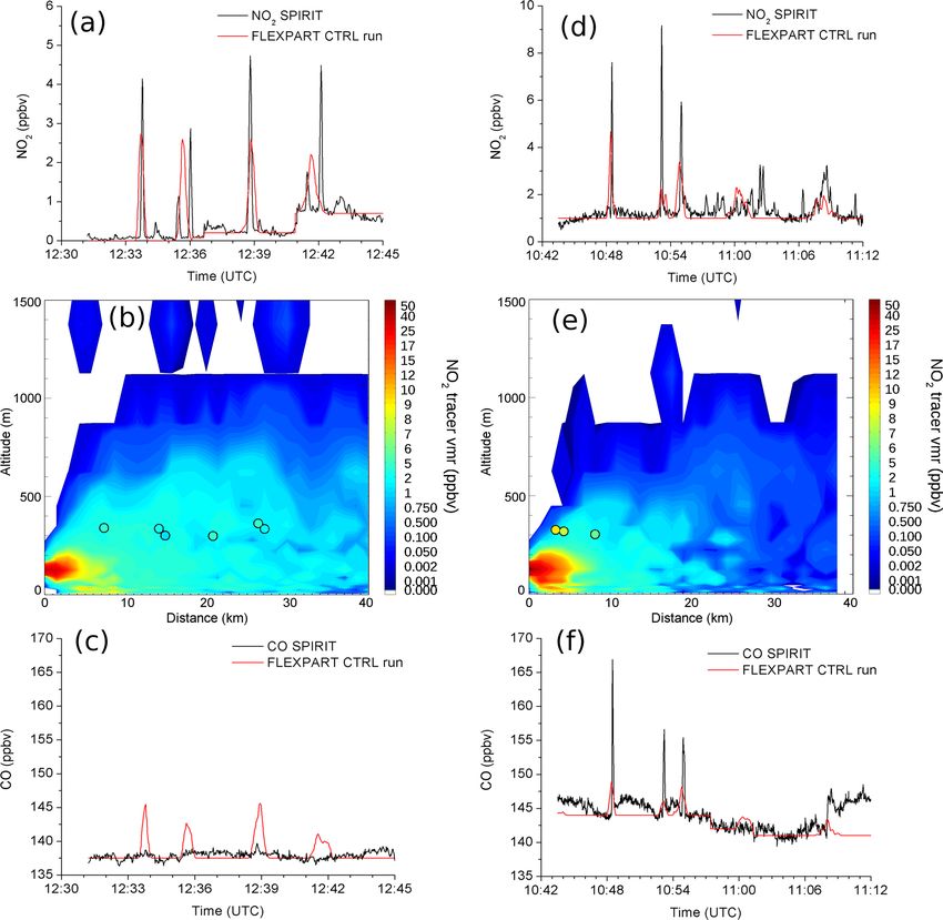
11402                                                                V. Brocchi et al.: Local air pollution from oil rig emissions

Africa; Knippertz et al., 2015) project conducted fieldwork           molecule abundance. The overall uncertainties are 4 ppbv for
in southern West Africa (SWA) in 2016 to investigate the im-          CO and 0.5 ppbv +5 % for NO2 at 1.6 s time resolution.
pact of anthropogenic emissions, notably on air quality. One             SO2 measurements are performed using a pulsed fluores-
part of the project included airborne measurements of flaring         cence SO2 analyser (Thermo Electron, Model 43C Trace
emissions in order to fill the data gap on oil extraction ac-         Level). Ultraviolet (UV) light is absorbed by SO2 molecules
tivities in SWA. Those in situ measurements are, as far as we         in the sample gas which become excited and subsequently
know, the first reported data on oil extraction activities in this    decay to a lower energy state. The emitted light is detected
region.                                                               by a photomultiplier tube and is proportional to the SO2 con-
   We use here the Lagrangian transport model FLEXPART                centration in the sample gas. The time resolution of the mea-
(FLEXible PARTicle dispersion model; Stohl et al., 2005)              surements is 1 s, with a moving average of 30 s to smooth the
in combination with an inventory of emissions dedicated to            data. The lower detection limit is 0.315 ppbv. The instrument
flaring emissions and created in the framework of the DAC-            was multipoint calibrated before and after the campaign.
CIWA project (Deetz and Vogel, 2017) to reproduce the air-               Total aerosol concentrations were measured with
craft measurements. We focus on evaluating the sensitivity            a butanol-based condensation particle counter (CPC;
of the model to two parameters: the emission flux and the in-         CPC TSI 3010, modified for aircraft use; Schröder and
jection height of the flaring emissions. After a brief descrip-       Ström, 1997; Fiebig et al., 2005). The particle counter was
tion of the DACCIWA project and the platform in Sect. 2, we           mounted inside the fuselage behind the Falcon isokinetic
present in Sect. 3 the model and the flaring emission inven-          aerosol inlet. The large particle cut-off diameter imposed
tory we used as well as the estimation of the flaring plume           by the inlet has been found to be between 1.5 and 3 µm,
injection height. We discuss the modelling results in Sect. 4.        depending on flight altitude (Fiebig, 2001). The lower
                                                                      cut-off diameter of the CPC was at ∼ 10 nm. Particle losses
                                                                      due to diffusion effects were minimised by using a standard
                                                                      5.75 L min−1 bypass flow to the instrument. Using the
2     The DACCIWA–APSOWA project                                      particle loss calculator described in von der Weiden et
                                                                      al. (2009), we estimate the particle losses in the tubing to be
2.1    Description of the campaign                                    less than 10 % for the relevant size range. Flight sequences
                                                                      inside clouds are known to cause sampling artefacts and
The EU-funded project DACCIWA focuses on the coupling                 have therefore been removed from the dataset.
between dynamics, aerosols, chemistry and clouds (Flamant
et al., 2017). The research campaign was set up in June–              2.2   Flight planning and FPSO description
July 2016 and undertook activities ranging from airborne
measurements to running atmospheric numerical models. A               The first floating production storage and offloading (FPSO)
map showing the location of the research site is presented in         vessels were installed in Indonesia in 1974. Since this year,
the Supplement (Fig. S1).                                             their number has steadily increased (Shimamura, 2002). The
   Our Atmospheric Pollution from Shipping and Oil Plat-              concept of those platforms based on ship structure makes the
forms of West Africa (APSOWA) project complementing                   development of small-size oil fields and the exploitation of
DACCIWA seeks to characterise gaseous and particulate pol-            them further from the coast and thus in deeper water pos-
lutants emitted by oil platforms off the coast of the Gulf            sible (Shimamura, 2002). Those platforms have other ad-
of Guinea by dedicated flights conducted with the DLR                 vantages (Shimamura, 2002): they are faster to build than
(Deutsches Zentrum für Luft- und Raumfahrt) research air-             other floating structures, they have inbuilt storage capability
craft Falcon 20. Different instruments for gas and partic-            and thus do not necessitate pipelines, and they are movable
ulate measurements were deployed onboard. We focus on                 and easily implantable on another oil field. Because of all
CO, NO2 , SO2 and aerosol measurements during two flights             those reasons, the FPSO systems will continue to develop.
on 10 and 14 July. Both CO and NO2 were measured                      Among the techniques used to dispose of the gas associated
by SPIRIT (SPectromètre InfraRouge In situ Toute alti-                with the crude oil extraction, one is the flaring, consisting
tude; Catoire et al., 2017). This infrared absorption spec-           of burning the gas in an open flame through a stack. This
trometer uses continuous-wave distributed-feedback room-              leads to a mixture of emitted gases which can reach the free
temperature quantum cascade lasers (QCLs) allowing on-                troposphere if the meteorological conditions are favourable
line scanning of mid-infrared rotational–vibrational lines            (Fawole et al., 2016b). The two targeted flights, on 10 and
with spectral resolution of 10−3 cm−1 . In the present cam-           14 July, consisted of about 3–4 h of meandering transects
paign, the ambient air is sampled in a multipass cell with            through emission plumes in the MBL about 300 m a.s.l.) off
a path length of 134.22 m and in micro-windows around                 the coast of West Africa, from Côte d’Ivoire to Togo. We
the 2179.772 cm−1 line for CO and the 1630.326 cm−1 line              focus on the flights in the vicinity of the FPSO Kwame
for NO2 . A home-made software using the HITRAN 2012                  Nkrumah platform, on the Jubilee Field, off the coast of
database (Rothman et al., 2013) is used to deduce the total           Ghana (4◦ 350 47.04 N, 2◦ 530 21.11 W). It measures 330 m in

Atmos. Chem. Phys., 19, 11401–11411, 2019                                             www.atmos-chem-phys.net/19/11401/2019/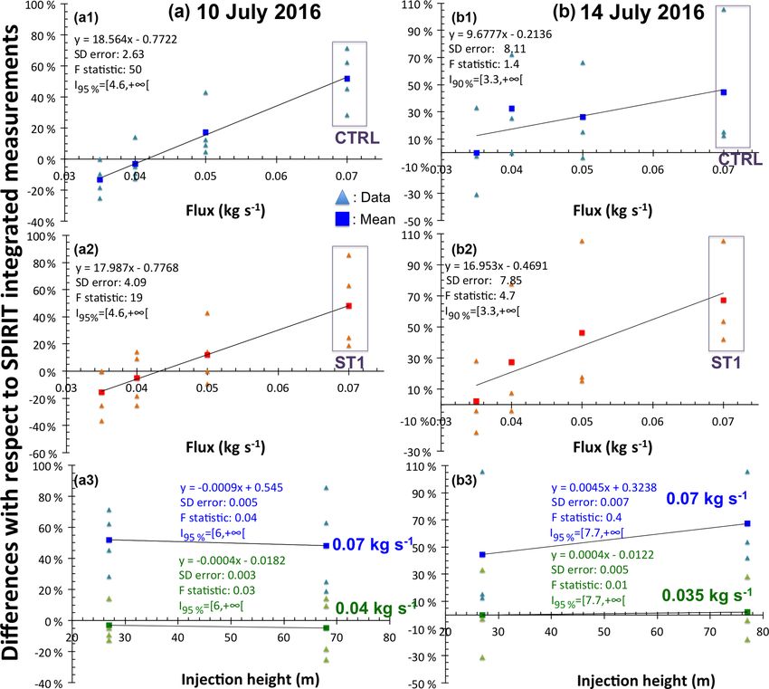
V. Brocchi et al.: Local air pollution from oil rig emissions                                                             11403

length by 65 m in width, and its height up to the top of the    of the species. The CO, SO2 and NO2 fluxes estimated with
chimney is estimated to be 112 m a.s.l. During the campaign,    this method for our 2 d of interest for the FPSO platform are
no contact with this FPSO could be obtained in order to have    1.1 × 10⁻¹ , 4.23 × 10⁻⁵ and 7 × 10⁻² kg s−1 , respectively.
more information on its functioning.                            Note that the highest uncertainties (+33 %; −79 %) associ-
                                                                ated to the estimation of gas-flaring emissions arise from the
                                                                parameters required in the combustion equations, e.g. the gas
3     Method                                                    composition, the source temperature and the flare character-
                                                                istics.
3.1    Lagrangian particle dispersion modelling

The Lagrangian model FLEXPART (Stohl et al., 2005) is
                                                                3.3   Estimation of the flaring plume injection height
used to study the transport of the emitted plume from the
FPSO in the MBL. It simulates long-range transport and
dispersion of atmospheric tracers released over time by         The oil flaring emissions are generally emitted at higher tem-
computing trajectories of a large number of tracer parti-       peratures than the temperature of the surrounding environ-
cles. Model calculations are based on meteorological data       ment, which implies an important role for the buoyancy at the
from the European Centre for Medium-Range Weather Fore-         stack exit. Indeed, the buoyancy corresponds to a density ra-
casts (ECMWF), ERA-INTERIM L137 (Dee et al., 2011),             tio between the air parcel and its colder surrounding environ-
extracted every 3 h and with a horizontal grid mesh size        ment and leads to the rise of this parcel under the influence
of 0.5◦ × 0.5◦ . The calculations are performed in forward-     of gravity. This effect is to be distinguished from the momen-
dispersion mode with the model version 9.0. The particles are   tum effect, defined as the product of an element mass by its
released with the chemical properties of NO2 , CO and SO2       velocity, which can be neglected for such a high-temperature
using constant emissions from the Deetz and Vogel (2017)        plume (Briggs, 1965). The buoyancy raises the plume above
inventory during 7 h, with a spin-up of 5 h, allowing the       its initial injection height and can lead to a source height that
model to be balanced independently from the initial condi-      can be several times higher than the real height of the stack
tions. During the simulation, the NO2 - and SO2 -like parti-    (Arya, 1999). The calculation required to determine the rise
cle mass is lost by wet and dry deposition and by OH re-        of a plume depends on the wind conditions and the atmo-
action (concentrations from GEOS-CHEM model; technical          spheric stability. Before determining those parameters, we
note FLEXPART v8.2, http://flexpart.eu/downloads/26, last       determine the MBL height that defines the part of the tro-
access: November 2018), which allows a lifetime of about        posphere in which we flew. The MBL is about 680 m a.s.l. on
3 h at 298 K in the MBL for NO2 . CO-like particle mass is      10 July and 582 m a.s.l. on 14 July, according to the Euro-
only lost by OH reaction.                                       pean (ECMWF) and US (NCEP) operational forecasts. The
                                                                wind conditions are determined by the Falcon 20 measure-
3.2    Flaring emission inventory                               ment system. An average of the wind speed measurements is
                                                                calculated during the flight period in the vicinity of the plat-
Our study is based on a new gas-flaring emission inven-
                                                                form (see Sect. 4.1). For 10 July, an 8 min mean wind speed
tory developed for the DACCIWA project (Deetz and Vo-
                                                                of 9.4 ± 0.5 m s−1 was calculated, where the standard devia-
gel, 2017). This inventory provides emissions of CO, CO2 ,
                                                                tion represents the natural variability, which is larger than the
NO, NO2 and SO2 for June–July 2014 and 2015, and we
                                                                measurement uncertainty. For 14 July, a 7 min wind speed
use a 2016 updated version for the period of the APSOWA–
                                                                mean of about 6.6 ± 0.7 m s−1 was calculated. Thus, for both
DACCIWA campaign. It is based on remote-sensing observa-
                                                                days the conditions are windy.
tions using VIIRS nighttime radiant heat in combination with
                                                                   Concerning the potential temperature for 10 and 14 July,
combustion equations from Ismail and Umukoro (2016). The
                                                                the atmosphere is considered to be stable with a positive po-
emission estimation method is described in detail in Deetz
                                                                tential temperature gradient. With the previous parameters
and Vogel (2017). Only the assumptions of interest for our
                                                                defined, it is possible to calculate the plume injection height
study are indicated: first, the natural gas composition in-
                                                                1H (in m) by using Eq. (1), reported by Briggs (1965, 1984):
cludes 0.03 % H2 S (Sonibare and Akeredolu, 2004). Sec-
ond, this composition measured in the Niger Delta is valid
for West Africa in general. Third, the source temperature is
deduced from the VIIRS measurements on a monthly mean.                   1/3
                                                                         Fb
For the FPSO platform, it is set to 1600 K, which is a good     1H = 2.6       ,                                             (1)
                                                                         us
order of magnitude, since the flame temperature can be as
high as 2000 K (Fawole et al., 2016b). Fourth, for such a
temperature, NO2 is considered to be a primary pollutant
coming from the rapid conversion of NO close to the source,     with Fb as the buoyancy effect (in m4 s−3 ) defined in Eq. (2),
and the inventory does not include any later transformation     u as the wind speed (in m s−1 ) and s as the stability parameter

www.atmos-chem-phys.net/19/11401/2019/                                        Atmos. Chem. Phys., 19, 11401–11411, 2019
11404 V. Brocchi et al.: Local air pollution from oil rig emissions
Table 1. Flux and injection height for the reference control run (CTRL) and for the sensitivity tests (STs) for each day of flight.
Run name Date of NO2 flux SO2 flux CO flux Injection height
flight (kg s−1 ) (kg s−1 ) (kg s−1 ) (m)
10 Jul 2016
CTRL 0.07 4.23 × 10⁻⁵ 0.11 27
14 Jul 2016
10 Jul 2016 68
ST1 0.07 Not included Not included
14 Jul 2016 77
10 Jul 2016
ST2 0.035–0.05 Not included Not included 27
14 Jul 2016
10 Jul 2016 68
ST3 0.035–0.05 Not included Not included
14 Jul 2016 77
(in s−2 ) defined in Eq. (3) (Briggs, 1965): will be performed to see the impact on the results of the in-
jection height in the model by using the injection height from
1T
Fb = g wr 2 , (2) VDI 3782 (1985).
Ts
g ∂T
s= + 0. (3)
T ∂z
4 Results and discussion
T , Ts , w and r are the absolute temperature of the ambient
air, the absolute temperature of the stack gases, the vertical 4.1 Description of the measurements
velocity of the effluent at the stack exit and the radius of
the stack, respectively. 1T is the difference between the two Figure 1 presents the part of the flights in the vicinity of
temperatures. In Eq. (3), g is the gravitational acceleration, the FPSO platform. During the flight on 10 July, the flaring
z the altitude and 0 the adiabatic lapse rate. Both the tem- plume was crossed several times (Fig. 1a). It led to four NO2
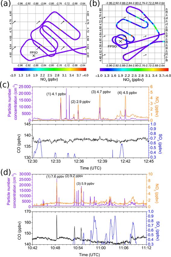
perature at the stack exit and the effluent velocity are taken peaks between 12:33 and 12:45 UTC at an altitude of around
from Deetz and Vogel (2017). The calculated plume injec- 300 m (Fig. 1c). Four simultaneous peaks of aerosols were
tion height 1H is 27 m for 10 and 14 July. Briggs’ algorithm measured (Fig. 1c). Neither simultaneous CO peaks (within
underestimates the plume rise in the stable atmospheric con- its lower detection limit, 0.3 ppbv; Catoire et al., 2017) nor
dition (Akingunola et al., 2018). Therefore, another method SO2 peaks (within its lower detection limit, 0.3 ppbv; see
has been tested to determine the injection height that is based Sect. 2.1) were detected in the plume of the FPSO platform
on VDI 3782 (1985). For a stable atmosphere, the injection for this flight. No peak was measured during a second series
height 1H (in m) of the plume is determined by Eq. (4): of transect at a higher altitude (around 600 m; Fig. 1a).
During the flight on 14 July, three NO2 peaks were mea-
1H = 74.4 × Q0.333 × u−0.333 , (4) sured during the first transects between 10:48 and 11:00 UTC
at around 300 m altitude downwind of the FPSO vessel
with u as the wind speed (in m s−1 ) and the unit of the co- (Fig. 1b). Those peaks were simultaneously measured with
efficient (74.4; in s4 kg−1 m−2 ). The heat flow Q (in units of aerosol and CO peaks (Fig. 1d), but still no SO2 peak was
MW) (Eq. 5) is defined in Deetz and Vogel (2017) as detected. Knowing that SO2 comes from H2 S combustion
1 (Sonibare and Akeredolu, 2004), these results suggest that
Q=H , (5) a gas composition of 0.03 % of H2 S induces an emission of
f
SO2 concentration lower than the detection limit of the in-
with H as the radiant heat observed by VIIRS (in units of strument from 3 km of our measurements or that the natural
MW) and f as the fraction of radiated heat set to 0.27 by gas composition given by Deetz and Vogel (2017) for the
Deetz and Vogel (2017) after having averaged the f values Niger Delta is different from that in Ghana for those two
given in Guigard et al. (2000). The calculated plume injection flights. The presence (or lack) of CO peaks is discussed in
heights are, according to Eq. (4), 68 and 77 m for 10 and Sect. 4.3.
14 July, respectively. Moreover, SPIRIT allows measurements every 1.6 s. Con-
The two methods of injection height calculation do not sidering the case on 10 July where we have the maximum air-
give similar results. The control run (CTRL; Table 1) will craft speed (118 m s−1 ) and the shortest peak (lasting about
use Briggs’ algorithm with an injection height of the parti- 16 s), the plume width is larger than the measurement e-fold
cles of 27 m for both days. A sensitivity test (ST1; Table 1) time multiplied by the flight speed. Thus, for all the narrow
Atmos. Chem. Phys., 19, 11401–11411, 2019 www.atmos-chem-phys.net/19/11401/2019/V. Brocchi et al.: Local air pollution from oil rig emissions 11405
Figure 1. (a) NO2 concentration as a function of the flight trajectory downwind of the FPSO plume for 10 July. The black arrows show the
wind direction (from ECMWF). (c) NO2 , aerosol, CO and SO2 concentrations as a function of time, restricted in a part of the flight trajectory
in (a). The peaks studied are labelled by a number (from 1 to 4). (b) and (d) are similar to (a) and (c) for 14 July.
peaks, the maximum plume concentration is real, not a plume 4.2 FLEXPART simulations of the flaring emissions
diluted with its surrounding environment.
In order to confirm that the peaks detected by the aircraft in-
struments correspond to the flaring emissions from the plat-
form and to simulate them, forward trajectories are calcu-
lated using FLEXPART. First, as a reference, a simulation
www.atmos-chem-phys.net/19/11401/2019/ Atmos. Chem. Phys., 19, 11401–11411, 201911406 V. Brocchi et al.: Local air pollution from oil rig emissions Figure 2. Left column: 10 July. (a) NO2 concentration as a function of time for SPIRIT measurements (black) and FLEXPART CTRL run simulation (red). (b) Vertical section of the simulated NO2 concentration (in vmr – volume mixing ratio with units of ppbv) in the plume (CTRL run) as a function of distance from the source and altitude. The coloured circles correspond to the measurement peaks. (c) CO concentration as a function of time for measurements (black) and FLEXPART CTRL run simulation (red). Right column: 14 July. (d), (e) and (f) similar to (a), (b) and (c). called CTRL is run in which the NO2 flux for the FPSO multaneously to the measured ones for oil facilities emissions platform is taken from Deetz and Vogel (2017), i.e. 7 × in the Norwegian Sea. A NO2 background concentration has 10−2 kg s−1 , and the injection height is 27 m, calculated been added to the last two peaks. This value is an average with Briggs’ method (see Sect. 3.3). A comparison of the of the measurements taken outside the plume and is repre- wind speed and direction between ECMWF simulations and sentative of the ambient pollution not taken into account in the Falcon measurements is presented in the Supplement. FLEXPART, as this model only simulates the pollution com- The wind speed and direction derived from ECMWF agree ing from the platform. Concerning the second and the fourth within 1 m s−1 and ∼ 1.8◦ , respectively, for 10 July (Fig. S2) peak (Fig. 2a), the measurements show two close peaks that and within ∼ 1 m s−1 and ∼ 7◦ , respectively, for 14 July FLEXPART cannot simulate individually, leading to a sin- (Fig. S3). So the transport is well reproduced in FLEXPART. gle and broader simulated peak. This is probably due to an Figure 2a compares observed and simulated time series of error in the dispersion modelling induced by the horizontal NO2 concentrations for the flight on 10 July. The four mea- and vertical wind field resolution that prevents us from com- sured peaks are all remarkably well reproduced in time by paring peak-to-peak concentrations. Even with a finer wind FLEXPART. Another study by Tuccella et al. (2017), using field grid mesh of 0.125◦ × 0.125◦ (simulation not shown), WRF-Chem, was able to reproduce the simulated peaks si- such close peaks cannot be distinguished, suggesting a still- Atmos. Chem. Phys., 19, 11401–11411, 2019 www.atmos-chem-phys.net/19/11401/2019/
V. Brocchi et al.: Local air pollution from oil rig emissions                                                               11407

insufficient spatial resolution. Instead, the integrated area un-   more measurements are needed at different altitudes and dis-
der each of the measured and simulated plume transects will         tances from the emission source.
be compared and presented in Fig. 3, with the percentages              Besides the weather conditions and the functioning of the
representing the relative differences with respect to SPIRIT        platform, the flight location is also an important parameter to
measurements. Figure 2d also compares the observed and              be able to evaluate our measurements. Figure 2b and e show
simulated NO2 concentrations for the flight of 14 July. The         the NO2 plume simulated with FLEXPART as a function
simulation gives three peaks concomitant with the three mea-        of distance from the source and altitude on 10 and 14 July,
sured peaks of interest.                                            respectively. The aircraft measurements, represented by the
   Comparisons between CTRL run and SPIRIT measure-                 coloured circles, are located at the upper part of the plume,
ments for both flights (Fig. 3a1 for 10 July; Fig. 3b1 for          away from the strongest concentrations. The work carried out
14 July) show that the simulated concentrations are always          is thus limited by the flight trajectories which were too high
overestimated for all the peaks (percentage larger than 0 %).       and too far from the FPSO platform to catch the part of the
Sensitivity tests are performed in order to show the FLEX-          plume with the highest concentrations. The operational con-
PART response to the flux. Fluxes lower than 0.07 kg s−1 are        ditions during the flights were complex for the pilots, and
tested from 0.035 to 0.05 kg s−1 . Figure 3a1 and b1 show           safety concerns forced us to respect a minimum flight level
the variations in the differences between the measurements          (300 m) and a minimum distance from the source. Finally,
and the FLEXPART simulations with the flux used in FLEX-            we found that the NO2 concentration difference between the
PART for the injection height from Briggs (1965). The plots         measurements and the simulations does not seem to depend
for both days show a linear response of FLEXPART to the             on the distance from the source, since the measurements are
flux increase, with a best estimation reached for 0.04 kg s−1       already too far.
for the flight on 10 July and 0.035 kg s−1 for the flight on           Emissions from oil and gas production vary depending on
14 July. Figure 3a2 and b2 show similar conclusions but             the operating conditions of the platforms, making them vari-
for the injection height from VDI 3782 (1985). To deter-            able and hard to analyse (Law et al., 2017). Considering this,
mine whether the observed linear relationship between the           it is possible to have sources of NOx (and SO2 if present)
percentages and the flux or the injection height occurs by          from non-flaring combustion processes like the power gen-
chance, a simple F test is performed, assuming that the vari-       eration for the facility (Villasenor et al., 2003). No review
ances are homogeneous and the results follow a Gaussian             can be found in the literature to estimate the magnitude of
distribution. F -statistic coefficients are calculated and com-     those emissions. As a comparison, during the ACCESS air-
pared to the 95 % or 90 % confidence interval with (1, N −2)        craft campaign (Tuccella et al., 2017) in the Arctic, the max-
(N: total number of results) as degrees of freedom (see val-        imum NOx mixing ratio associated to oil and gas platforms
ues in brackets [u; +∞] in Fig. 3). If the value F is included      is about 10 ppbv (Fig. 5 in Tuccella et al., 2017). For the AC-
in the confidence interval, then the relationship can be con-       CESS campaign, it is known that the facilities were operating
sidered to be linear. The standard errors on the slope are also     under normal conditions, and the flight altitude ranges from
added in the plots of Fig. 3.                                       120 to 250 m. The comparison of the FPSO in the Gulf of
   For the flight on 10 July, the standard error of the slope       Guinea with the platforms in Arctic shows that the NO2 mea-
coefficients and the F test (95 % confidence) show linear re-       sured during DACCIWA campaign is in the range of a normal
lationships between the percentage difference and the flux.         functioning mode. As mentioned in Zhang et al. (2019), the
Only the results on 14 July for the plot with the injec-            sources associated to non-flaring combustion are not always
tion height of VDI 3782 (1985, panel b2) show a positive            negligible, depending on the operating conditions. Thus, we
F test, but with 90 % confidence. No conclusions can be             cannot exclude a contribution from another NOx source over-
drawn for the results on 14 July with the injection height          estimating the results, but this contribution is not important
of Briggs (1965; Fig. 3b1). In order to show the response           when gas-flaring activity is in normal mode (Zhang et al.,
of FLEXPART to the injection height, Fig. 3a3 and b3 show           2019).
the percentages versus the injection height (Briggs, 1965, or          We can use the best simulation on each day to estimate
VDI 3782, 1985). FLEXPART shows similar results regard-             the percentage of pollutants transported inside and above the
less of the injection height used as input whatever the flux        MBL. In both cases, about 90 % of the pollutants stay in-
used. All the cases show standard error on the slope coeffi-        side the MBL and are able to impact the population living
cients larger than the slope itself and an F value not included     along the coastline. Measurements made along the coastline
in the confidence interval (at 95 % confidence, as shown in         have shown that NO2 concentrations are generally greater
the figure, and even 90 %, not shown). These results suggest        than 2 ppb for suburban sites and greater than 20 ppb near
that the differences between the two injection heights are not      industrial sites (Bahino et al., 2018). Given the wind velocity
significant enough with respect to the vertical resolution of       (from 6.6 to 9.4 m s−1 ), the air masses attain the coast in 2
the model or that the measurements are too far to be influ-         to 3 h, which does not allow the transport of significant NO2
enced by the changes in this parameter. However, to really          concentrations to impact air quality in this area. This is con-
conclude about the injection height and to evaluate the flux,       firmed when looking at FLEXPART simulations in Fig. 2b

www.atmos-chem-phys.net/19/11401/2019/                                            Atmos. Chem. Phys., 19, 11401–11411, 2019
11408                                                                      V. Brocchi et al.: Local air pollution from oil rig emissions

Figure 3. Differences (in %) between FLEXPART simulations and SPIRIT integrated measurements depending on flux or injection height
used as input in the model for (a) the flight on 10 July and (b) the flight on 14 July. Panels (a1) and (b1) represent the change in the percentage
with the flux by using the injection height from Briggs’ algorithm (1965; blue data; i.e. 27 m) and panels (a2) and (b2) with injection height
from VDI 3782 (1985; orange data; i.e. 68 m – a2 – or 77 m – b2). Panels (a3) and (b3) represent the change in the percentage with the
injection height for the flux from Deetz and Vogel (2017; blue data; 0.07 kg s−1 ) and for the flux used in the sensitivity tests (green data;
0.04 kg s−1 for 10 July in a3 and 0.035 kg s−1 for 14 July in b3). For all panels, triangles represent the data for all the peaks measured and
squares represent the mean from these data. The slope, standard error values for the slope coefficients, the F statistic and the confidence
interval (I95 % or I90 % only for panel b1 and b2) are added for all the plots.

and e. They show that NO2 concentrations are already very                   ulates four CO peaks concomitant with the four NO2 peaks,
low (< 1 ppbv) from 40 km from the source on 10 July and                    while no increase in CO was observed. On 14 July, three
even closer (from 20 km from the source) on 14 July. With                   peaks of CO are simulated at the same time as the three mea-
the distance between the coast and the emission source fol-                 sured ones but are underestimated. CO is always included as
lowing the wind direction being 70 km, only pollutants with                 a gas emitted from flaring in the inventory for this specific
a relatively long lifetime or secondary pollutant like O3 can               vessel, while it does not seem to be the case each time. A
impact the air quality of the coast.                                        discussion on the flaring combustion processes is presented
   Considering the very low SO2 flux, the FLEXPART simu-                    below.
lations in the CTRL run induce insignificant SO2 concentra-
tion at an aircraft-sampled location (results not shown).                   4.3   Combustion processes involved in oil flare
   We performed CO simulations, as CO peaks were mea-
sured in one case out of two (Fig. 2c and f). For those                     From a combustion point of view, flares generate non-
simulations, we used the injection height of 27 m of the                    premixed highly turbulent flames, characterised by high-
CTRL run and the flux from Deetz and Vogel (2017) of                        frequency fluctuating flow fields. Flares can be air-assisted
1.1×10⁻¹ kg s−1 . For the flight on 10 July, FLEXPART sim-                  or steam-assisted in order to achieve a better efficiency. The

Atmos. Chem. Phys., 19, 11401–11411, 2019                                                     www.atmos-chem-phys.net/19/11401/2019/
V. Brocchi et al.: Local air pollution from oil rig emissions                                                                   11409

turbulence increases the mixing and affects the chemical re-     mainly inside the MBL, limiting the transport to the coastline
action process. Very recent attempts to model such flames        located 70 km downwind of the FPSO.
(Aboje et al., 2017; Damodara et al. 2017) showed that the          Sources of uncertainties are associated with the different
influence of the composition of the natural gas and the valid-   calculations and hypotheses, but the work is mainly limited
ity of the chemical kinetic mechanism are of primary im-         by the flight trajectories that are too far and too high from the
portance in predicting the emitted species. Moreover, the        platform. So it remains necessary to better quantify the emis-
flame characteristics, such as temperature, height and length,   sions released during the flaring processes locally but also at
have a strong impact on the dispersion of the plume together     wider scales. Generally speaking, this study suggests that for
with wind speed and other meteorological variables (Rah-         flights planned in the heart of a flaring plume, it should be
nama and De Visscher, 2016). All these parameters need to        possible to link the flaring observations obtained by satellites
be taken into account when considering air field campaigns.      with the emissions deduced from the airborne measurements.
   McDaniel (1983) clearly demonstrated that CO emissions        If this relationship is possible, a general relationship between
are strongly related to flare efficiency. When the efficiency    the emissions and the radiant heat could thus allow estimat-
is ca. 99.8 %, CO is below 10 ppmv (Fig. A-5 in McDaniel,        ing the emissions of all flaring processes detected by satellite.
1983), while CO emissions may reach 440 ppmv when the
efficiency drops to 64 % (Fig. A-8 in McDaniel, 1983). CO
emissions can clearly be linked to the quality of the com-       Data availability. The aircraft data used here can be accessed us-
bustion, which is directly impacted by the turbulence. The       ing the DACCIWA database at http://baobab.sedoo.fr/DACCIWA/
observed difference between 10 and 14 July in terms of CO        (last access: October 2018; Brissebrat et al., 2017). A 2-year em-
emissions mostly lies in the different wind conditions be-       bargo period applies after the upload. External users can request the
                                                                 release of datasets before the end of the embargo period.
tween these 2 d. First, the wind speed was lower on 14 July,
which makes less O2 available to burn with natural gas; sec-
ond, it appears that the wind direction was not clearly estab-
                                                                 Supplement. The supplement related to this article is available on-
lished, as can be seen from the much more dispersed plume in     line at: https://doi.org/10.5194/acp-19-11401-2019-supplement.
Fig. 1b, resulting in incomplete combustion pockets favour-
ing CO formation. However, a decrease in efficiency should
also lead to lower temperatures and NOx emissions, which is      Author contributions. HS was the mission scientist for the Falcon
not observed here. The results of this campaign would re-        20 aircraft and VC the principal investigator (PI) of the EUFAR2–
quire analysis in the light of computational fluid dynamic       APSOWA campaign. VC, SC and VB participated in the SPIRIT
simulations, accounting for a realistic natural gas composi-     measurements aboard the aircraft, with remote assistance from CR
tion and its high-temperature chemistry, which are beyond        for the SPIRIT maintenance. VB, GS and DS performed flight data
the scope of this study.                                         analyses for their respective instruments. KD provided the updated
                                                                 version of his inventory for the period of the campaign and the VDI
                                                                 report. AD performed simulations using WRF-Chem to simulate the
                                                                 FPSO plume and gave advice for the modelling method. GK and VB
5   Conclusions
                                                                 performed the FLEXPART simulations. GD conducted the combus-
                                                                 tion part of the paper. VB wrote the paper, with contributions from
This study was conducted in the framework of the DAC-            all co-authors.
CIWA FP7 European project in July 2016 in southern West
Africa. One target of the project was to measure emissions
from oil rigs, which were not well estimated until then. With    Competing interests. The authors declare that they have no conflict
two flights planned in the vicinity of a FPSO platform, we       of interest.
reported the first flaring in situ measurements in this re-
gion. The aim of this work was to evaluate the capacity of
the FLEXPART model to reproduce the NO2 airborne mea-            Special issue statement. This article is part of the special issue “Re-
surements and to evaluate the inventory of Deetz and Vogel       sults of the project ‘Dynamics-aerosol-chemistry-cloud interactions
(2017) in the case of point sources of pollution such as oil     in West Africa’ (DACCIWA) (ACP/AMT inter-journal SI)”. It is not
platforms. The injection height of the plume was estimated       associated with a conference.
by performing different calculations. According to several
sensitivity runs, it appears that the emission flux given by
Deetz and Vogel (2017) overestimates the concentrations,         Acknowledgements. We thank Patrick Jacquet for instrumental sup-
whereas a lower NO2 flux roughly reproduces the measure-         port before and during the campaign. The DLR crew is acknowl-
ments. Concerning the injection height, the sensitivity tests    edged for flying operations. This work was funded by the EU
                                                                 FP7 EUFAR2 Transnational Access project and DACCIWA project
are not conclusive, showing the need for more and better-
                                                                 (grant agreement no. 603502), the Labex VOLTAIRE (ANR-10-
targeted measurements. An estimation of the pollutant distri-    LABX-100-01), the PIVOTS project provided by the Région Cen-
bution above or inside the MBL shows that the pollutants stay

www.atmos-chem-phys.net/19/11401/2019/                                           Atmos. Chem. Phys., 19, 11401–11411, 2019
11410 V. Brocchi et al.: Local air pollution from oil rig emissions
tre – Val de Loire (ARD 2020 programme and CPER 2015–2020) – Brissebrat, G., Belmahfoud, N., Cloché, S., Ferré, H., Fleury, L.,
and the APSOWA project from the INSU-LEFE-CHAT programme. Mière, A., and Ramage, K.: The BAOBAB data portal and DAC-
We thank Francesco Contino (Vrije Universiteit Brussel, Belgium) CIWA database, 19th EGU General Assembly, EGU2017, 23–
for the work undertaken on the simulations of flame. We also 28 April, 2017, Vienna, Austria, p. 4685, available at: http:
thank Gaëlle De Coetlogon and Alain Weill (Laboratoire Atmo- //baobab.sedoo.fr/DACCIWA/ (last access: July 2018), 2017.
sphères, Milieux, Observations Spatiales – Université Paris-Saclay Catoire, V., Robert, C., Chartier, M., Jacquet, P., Guimbaud, C.,
and CNRS, France) for their help in determining the MBL height. and Krysztofiak, G.: The SPIRIT airborne instrument: a three-
channel infrared absorption spectrometer with quantum cascade
lasers for in situ atmospheric trace-gas measurements, Appl.
Financial support. This work was funded by the EU FP7 EUFAR2 Phys. B., 123, 244, https://doi.org/10.1007/s00340-017-6820-x,
Transnational Access project and DACCIWA project (grant agree- 2017.
ment no. 603502), the Labex VOLTAIRE (ANR-10-LABX-100- Damodara, V., Chen, D. H., Lou, H. H., Rasel, K. M. A., Richmond,
01), the PIVOTS project provided by the Région Centre – Val de P., Wang, A., and Li, X.: Reduced combustion mechanism for
Loire (ARD 2020 programme and CPER 2015–2020) – and the AP- C1 –C4 hydrocarbons and its application in computational fluid
SOWA project from the INSU-LEFE-CHAT programme. dynamics flare modelling, J. Air Waste Manage., 67, 599–612,
https://doi.org/10.1080/10962247.2016.1268546, 2017.
Dee, D. P., Uppala, S. M., Simmons, A. J., Berrisford, P., Poli,
Review statement. This paper was edited by Mathew Evans and re- P., Kobayashi, S., Andrae, U., Balmaseda, M. A., Balsamo, G.,
viewed by Joseph Pitt and one anonymous referee. Bauer, P., Bechtold, P., Beljaars, A. C. M., van de Berg, L., Bid-
lot, J., Bormann, N., Delsol, C., Dragani, R., Fuentes, M., Geer,
A. J., Haimberger, L., Healy, S. B., Hersbach, H., Hólm, E. V.,
Isaksen, L., Kållberg, P., Köhler, M., Matricardi, M., McNally,
A. P., Monge-Sanz, B. M., Morcrette, J.-J., Park, B.-K., Peubey,
References C., de Rosnay, P., Tavolato, C., Thépaut, J.-N., and Vitart, F.: The
ERA-Interim reanalysis: configuration and performance of the
Aboje, A. A., Hughes, K. J., Ingham, D. B., Ma, L., Williams, A., data assimilation system, Q. J. Roy. Meteor. Soc., 137, 553–597,
and Pourkashanian, M.: Numerical study of a wake-stabilized https://doi.org/10.1002/qj.828, 2011.
propane flame in a cross-flow of air, Journal of Energy Institute, Deetz, K. and Vogel, B.: Development of a new gas-flaring emission
90, 145–158, https://doi.org/10.1016/j.joei.2015.09.002, 2017. dataset for southern West Africa, Geosci. Model Dev., 10, 1607–
Akingunola, A., Makar, P. A., Zhang, J., Darlington, A., Li, S.-M., 1620, https://doi.org/10.5194/gmd-10-1607-2017, 2017.
Gordon, M., Moran, M. D., and Zheng, Q.: A chemical trans- Elvidge, C. D., Zhizhin, M., Hsu, F.-C., and Baugh, K. E.: VI-
port model study of plume-rise and particle size distribution for IRS Nightfire: Satellite Pyrometry at Night, Remote Sensing, 5,
the Athabasca oil sands, Atmos. Chem. Phys., 18, 8667–8688, 4423–4449, https://doi.org/10.3390/rs5094423, 2013.
https://doi.org/10.5194/acp-18-8667-2018, 2018. Elvidge, C. D., Zhizhin, M., Baugh, K., Hsu, F.-C., and Ghosh, T.:
Anomohanran, O.: Determination of greenhouse gas emission re- Methods for Global Survey of Natural Gas Flaring from Vis-
sulting from gas flaring activities in Nigeria, Energy Policy, 45, ible Infrared Imaging Radiometer Suite Data, Energies, 9, 14,
666–670, https://doi.org/10.1016/j.enpol.2012.03.018, 2012. https://doi.org/10.3390/en9010014, 2015.
Arya, S. P.: Air Pollution Meteorology and Dispersion, Oxford Uni- Fawole, O. G., Cai, X., Levine, J. G., Pinker, R. T., and
versity Press, Department of Marine, Earth, and Atmospheric MacKenzie, A. R.: Detection of a gas flaring signature in the
Sciences, North Carolina State University, 1999. AERONET optical properties of aerosols at a tropical station
Asuoha, A. N. and Osu Charles, I.: Seasonal variation of meteoro- in West Africa, J. Geophys. Res.-Atmos., 121, 2016JD025584,
logical factors on air parameters and the impact of gas flaring on https://doi.org/10.1002/2016JD025584, 2016a.
air quality of some cities in Niger Delta (Ibeno and its environs), Fawole, O. G., Cai, X.-M., and MacKenzie, A. R.: Gas
African Journal of Environmental Science and Technology, 9, flaring and resultant air pollution: A review focus-
218–227, https://doi.org/10.5897/AJEST2015.1867, 2015. ing on black carbon, Environ. Pollut., 216, 182–197,
Bahino, J., Yoboué, V., Galy-Lacaux, C., Adon, M., Akpo, A., https://doi.org/10.1016/j.envpol.2016.05.075, 2016b.
Keita, S., Liousse, C., Gardrat, E., Chiron, C., Ossohou, M., Fiebig, M.: Das troposphärische Aerosol in mittleren Breiten –
Gnamien, S., and Djossou, J.: A pilot study of gaseous pollu- Mikrophysik, Optik und Klimaantrieb am Beispiel der Feldstudie
tants’ measurement (NO2 , SO2 , NH3 , HNO3 and O3 ) in Abid- LACE 98, PhD thesis, Ludwig-Maximilians-Universität, Institut
jan, Côte d’Ivoire: contribution to an overview of gaseous pol- für Physik der Atmosphäre, DLR, Oberpfaffenhofen, 2001.
lution in African cities, Atmos. Chem. Phys., 18, 5173–5198, Fiebig, M., Stein, C., Schroder, F., Feldpausch, P., and Petzold, A.:
https://doi.org/10.5194/acp-18-5173-2018, 2018. Inversion of data containing information on the aerosol particle
Briggs, G. A.: A Plume Rise Model Compared with Observations, size distribution using multiple instruments, J. Aerosol Sci., 36,
Journal of the Air Pollution Control Association, 15, 433–438, 1353, https://doi.org/10.1016/j.jaerosci.2005.01.004, 2005.
https://doi.org/10.1080/00022470.1965.10468404, 1965. Flamant, C., Knippertz, P., Fink, A. H., Akpo, A., Brooks, B., Chiu,
Briggs, G. A.: Plume rise and buoyancy effects, atmospheric C. J., Coe, H., Danuor, S., Evans, M., Jegede, O., Kalthoff,
sciences and power production, in: DOE/TIC-27601 N., Konaré, A., Liousse, C., Lohou, F., Mari, C., Schlager,
(DE84005177), edited by: Randerson, D., TN, Technical H., Schwarzenboeck, A., Adler, B., Amekudzi, L., Aryee, J.,
Information Center, U.S. Dept. of Energy, Oak Ridge, USA, Ayoola, M., Batenburg, A. M., Bessardon, G., Borrmann, S.,
327–366, 1984.
Atmos. Chem. Phys., 19, 11401–11411, 2019 www.atmos-chem-phys.net/19/11401/2019/V. Brocchi et al.: Local air pollution from oil rig emissions 11411 Brito, J., Bower, K., Burnet, F., Catoire, V., Colomb, A., Den- lar spectroscopic database, J. Quant. Spectrosc. Ra., 130, 4–50, jean, C., Fosu-Amankwah, K., Hill, P. G., Lee, J., Lothon, M., https://doi.org/10.1016/j.jqsrt.2013.07.002, 2013. Maranan, M., Marsham, J., Meynadier, R., Ngamini, J., Rosen- Schröder, F. and Ström, J.: Aircraft measurements of sub mi- berg, P., Sauer, D., Smith, V., Stratmann, G., Taylor, J. W., crometer aerosol particles (> 7 nm) in the midlatitude free Voigt, C., and Yoboué, V.: The Dynamics-Aerosol-Chemistry- troposphere and tropopause region, Atmos. Res., 44, 333, Cloud Interactions in West Africa field campaign: Overview https://doi.org/10.1016/S0169-8095(96)00034-8, 1997. and research highlights, B. Am. Meteorol. Soc., 99, 83–104, Shimamura, Y.: FPSO/FSO: State of the art, J. Mar. Sci. Technol., https://doi.org/10.1175/BAMS-D-16-0256.1, 2017. 7, 59–70, https://doi.org/10.1007/s007730200013, 2002. Guigard, S. E., Kindzierski, W. B., and Harper, N.: Heat Radia- Sonibare, J. A. and Akeredolu, F. A.: A theoretical pre- tion from Flares. Report prepared for Science and Technology diction of non-methane gaseous emissions from nat- Branch, Alberta Environment, ISBN 0-7785-1188-X, Edmonton, ural gas combustion, Energy Policy, 32, 1653–1665, Alberta, 2000. https://doi.org/10.1016/j.enpol.2004.02.008, 2004. Hassan, A. and Kouhy, R.: Gas flaring in Nigeria: Stohl, A., Forster, C., Frank, A., Seibert, P., and Wotawa, G.: Analysis of changes in its consequent carbon emis- Technical note: The Lagrangian particle dispersion model sion and reporting, Accounting Forum, 37, 124–134, FLEXPART version 6.2, Atmos. Chem. Phys., 5, 2461–2474, https://doi.org/10.1016/j.accfor.2013.04.004, 2013. https://doi.org/10.5194/acp-5-2461-2005, 2005. Ismail, O. S. and Umukoro, G. E.: Modelling combustion re- Tuccella, P., Thomas, J. L., Law, K. S., Raut, J.-C., Marelle, L., actions for gas flaring and its resulting emissions, Jour- Roiger, A., Weinzierl, B., Denier van der Gon, H.A.C., Schlager, nal of King Saud University – Eng. Sci., 28, 130–140, H., and Onishi, T.: Air pollution impacts due to petroleum extrac- https://doi.org/10.1016/j.jksues.2014.02.003, 2016. tion in the Norwegian Sea during the ACCESS aircraft campaign, Knippertz, P., Coe, H., Chiu, J. C., Evans, M. J., Fink, A. H., Elem. Sci. Anth., 5, 25, https://doi.org/10.1525/elementa.124, Kalthoff, N., Liousse, C., Mari, C., Allan, R. P., Brooks, 2017. B., Danour, S., Flamant, C., Jegede, O. O., Lohou, F., and VDI 3782: Dispersion of Air Pollutants in the Atmosphere, De- Marsham, J. H.: The DACCIWA Project: Dynamics–Aerosol– termination of Plume rise, Verein Deutscher Ingenieure, VDI- Chemistry–Cloud Interactions in West Africa, B. Am. Meteo- Richtlinien 3782 Part 3, 1985. rol. Soc., 96, 1451–1460, https://doi.org/10.1175/BAMS-D-14- Villasenor, R., Magdaleno, M., Quintanar, A., Gallardo, J. C., 00108.1, 2015. López, M., Jurado, R., Miranda, A., Aguilar, M., Melgarejo, Law, K. S., Roiger, A., Thomas, J. L., Marelle, L., Raut, J. C., L. A., Palmerín, E., Vallejo, C. J., and Barchet, W. R.: An air Dalsøren, S., Fuglestvedt, J., Tuccella, P., Weinzierl, B., and quality emission inventory of offshore operations for the explo- Schlager, H.: Local Arctic air pollution: Sources and impacts, ration and production of petroleum by the Mexican oil industry, Ambio, 46, 453–463, https://doi.org/10.1007/s13280-017-0962- Atmos. Environ., 37, 3713–3729, https://doi.org/10.1016/S1352- 2, 2017. 2310(03)00445-X, 2003. McDaniel, M.: Flare efficiency study, available at: http://www.epa. von der Weiden, S.-L., Drewnick, F., and Borrmann, S.: Particle gov/ttn/chief/ap42/ch13/related/ref_01c13s05_jan1995.pdf (last Loss Calculator – a new software tool for the assessment of the access: July 2018), 1983. performance of aerosol inlet systems, Atmos. Meas. Tech., 2, Nwankwo, C. N. and Ogagarue, D. O.: Effects of gas flaring on 479–494, https://doi.org/10.5194/amt-2-479-2009, 2009. surface and ground waters in Delta State Nigeria, Journal of Ge- Zhang, Y., Gautam, R., Zavala-Araiza, D., Jacob, D. J., Zhang, ology and Mining Research, 3, 131–136, 2011. R., Zhu, L., Sheng J.-X., and Scarpelli, T.: Satellite-observed Nwaugo, V. O., Onyeagba, R. A., and Nwahcukwu, N. C.: Effect of changes in Mexico’s offshore gas flaring activity linked gas flaring on soil microbial spectrum in parts of Niger Delta area to oil/gas regulations, Geophys. Res. Lett., 46, 1879–1888, of southern Nigeria, Afr. J. Biotechnol., 5, 1824–1826, 2006. https://doi.org/10.1029/2018GL081145, 2019. Osuji, L. C. and Avwiri, G. O.: Flared Gas and Other Pollutants Associated with Air quality in industrial Areas of Nigeria: An Overview, Chem. Biodivers., 2, 1277–1289, 2005. Rahnama, K. and De Visscher, A.: Simplified Flare Combustion Model for Flare Plume Rise Calculations, Can. J. Chem. Eng., 94, 1249–1261, 2016. Rothman, L. S., Gordon, I. E., Babikov, Y., Barbe, A., Chris Benner, D., Bernath, P. F., Birk, M., Bizzocchi, L., Boudon, V., Brown, L. R., Campargue, A., Chance, K., Cohen, E. A., Coudert, L. H., Devi, V. M., Drouin, B. J., Fayt, A., Flaud, J.-M., Gamache, R. R., Harrison, J. J., Hartmann, J.-M., Hill, C., Hodges, J. T., Jacquemart, D., Jolly, A., Lamouroux, J., Le Roy, R. J., Li, G., Long, D. A., Lyulin, O. M., Mackie, C. J., Massie, S. T., Mikhailenko, S., Müller, H. S. P., Nau- menko, O. V., Nikitin, A. V., Orphal, J., Perevalov, V., Per- rin, A., Polovtseva, E. R., Richard, C., Smith, M. A. H., Starikova, E., Sung, K., Tashkun, S., Tennyson, J., Toon, G. C., Tyuterev, V. G., and Wagner, G.: The HITRAN2012 molecu- www.atmos-chem-phys.net/19/11401/2019/ Atmos. Chem. Phys., 19, 11401–11411, 2019
You can also read