Discriminative Models for Multi-Class Object Layout
←
→
Page content transcription
If your browser does not render page correctly, please read the page content below
Int J Comput Vis
DOI 10.1007/s11263-011-0439-x

Discriminative Models for Multi-Class Object Layout
Chaitanya Desai · Deva Ramanan · Charless C. Fowlkes

Received: 2 March 2010 / Accepted: 18 March 2011
© Springer Science+Business Media, LLC 2011

Abstract Many state-of-the-art approaches for object rec-         of training images. We show state-of-the-art results on the
ognition reduce the problem to a 0-1 classification task. This    PASCAL VOC benchmark that indicate the benefits of
allows one to leverage sophisticated machine learning tech-       learning a global model encapsulating the spatial layout of
niques for training classifiers from labeled examples. How-       multiple object classes (a preliminary version of this work
ever, these models are typically trained independently for        appeared in ICCV 2009, Desai et al., IEEE international
each class using positive and negative examples cropped           conference on computer vision, 2009).
from images. At test-time, various post-processing heuris-
tics such as non-maxima suppression (NMS) are required            Keywords Object recognition · Context · Structured
to reconcile multiple detections within and between differ-       prediction · Cutting plane
ent classes for each image. Though crucial to good perfor-
mance on benchmarks, this post-processing is usually de-
fined heuristically.                                              1 Introduction
    We introduce a unified model for multi-class object
recognition that casts the problem as a structured prediction     A contemporary and successful approach to object recog-
task. Rather than predicting a binary label for each image        nition is to formulate it as a classification task, e.g. “Does
window independently, our model simultaneously predicts a         an image window at location i contain a given object o?”.
structured labeling of the entire image (Fig. 1). Our model       The classification formulation allows immediate applica-
learns statistics that capture the spatial arrangements of var-   tion of a variety of sophisticated machine learning tech-
ious object classes in real images, both in terms of which        niques in order to learn optimal detectors from training data.
arrangements to suppress through NMS and which arrange-           Such methods have the potential to encapsulate those sub-
ments to favor through spatial co-occurrence statistics.          tle statistical regularities of the visual world which sep-
    We formulate parameter estimation in our model as a           arate object from background. As a result, learning ap-
max-margin learning problem. Given training images with           proaches have often yielded detectors that are more robust
ground-truth object locations, we show how to formu-              and accurate than their hand built counterparts for a range
late learning as a convex optimization problem. We em-            of applications, from edge and face detection to general
ploy the cutting plane algorithm of Joachims et al. (Mach.        purpose object recognition (see e.g., Rowley et al. 1996;
Learn. 2009) to efficiently learn a model from thousands          Viola and Jones 2004).
                                                                      In contrast to the well founded techniques used for clas-
                                                                  sification of individual image patches, the problem of cor-
C. Desai () · D. Ramanan · C.C. Fowlkes
Department of Computer Science, UC Irvine, Irvine, CA, USA
                                                                  rectly detecting and localizing multiple objects from multi-
e-mail: desaic@ics.uci.edu                                        ple classes within an image of a scene has generally been
D. Ramanan
                                                                  approached in a far more ad-hoc manner. For example, non-
e-mail: dramanan@ics.uci.edu                                      max suppression (NMS) is required to remove some detec-
C.C. Fowlkes
                                                                  tions returned by a classifier based on overlap criteria or
e-mail: fowlkes@ics.uci.edu                                       more complicated heuristics (e.g. the mode finding approach
Int J Comput Vis
Table 1 A taxonomy of interactions captured in our model. Within a
single object class, our model can favor typical spatial layouts of ob-
jects (people often stand in crowds) while directly learning how to in-
hibit overlapping detections in such cases (NMS). Our model also cap-
tures long-range interactions between objects, such as the constraint
that there exists at most one object instance (counting). Analogous in-
teractions exist between object classes, including typical spatial rela-
tions between objects (bottles sit on tables), mutual exclusion (dog and
cat detectors should not respond to the same image region), and co-
occurrence (couches and cars do not commonly co-occur)
Fig. 1 Our framework. Classification-based approaches for recogni- Within-class Between-class
tion predict a binary label for a cropped window (left). We formulate
the recognition problem as predicting a sparse, structured label vector Activation Textures of objects Spatial cueing
specifying which windows, if any, contain particular objects in an en- Inhibition NMS Mutual exclusion
tire input image. The latter allows our model to capture a wide range of
contextual constraints among objects as described in Table 1 and Fig. 2 Global Expected counts Co-occurrence
NMS is generally described in terms of intra-class inhi-
bition, but can be generalized to suppression of overlapping
detections between different classes. We refer to this more
general constraint, that two objects cannot occupy the same
3D volume at the same time, as mutual exclusion. As seen
in a 2D image projection, the exact nature of this constraint
depends on the object classes. Figure 2 (right) shows an ex-
ample of ground-truth labelings in the PASCAL VOC (Ever-
Fig. 2 Our novel contributions include the ability to learn inhibitory
intra-class constraints (NMS) and inhibitory inter-class constraints ingham et al. 2007) dataset in which strict mutual-exclusion
(Mutual Exclusion) in a single unified model along with contextual would produce sub-optimal performance.
cuing and spatial co-occurrence. Naïve methods for NMS or mutual Object detections can also serve to enhance rather than
exclusion may fail for objects that tend to overlap themselves (left) inhibit other detections within a scene. This has been an
and other objects (right). In contrast, our framework learns how best
to enforce such constraints from training data. We formulate the tasks area of active research in object recognition over the last
of NMS and Mutual Exclusion using the language of structured pre- few years (Torralba et al. 2004; Murphy et al. 2003; Gal-
diction. This allows us to compute an optimal model by minimizing a leguillos et al. 2008; He et al. 2004; Hoiem et al. 2008;
convex objective function Baur et al. 2008; Kumar and Hebert 2005). For example,
different object classes may be likely to co-occur in a par-
of Dalal and Triggs 2005). Such tricks of the trade are essen- ticular spatial layout. People ride on bikes, bottles rest on
tial to good performance on benchmarks designed to penal- tables, and so on. In contextual cueing, a confident de-
ize multiple non-localized detections, however, they high- tection of one object (a bike) provides evidence that in-
light a clear disconnect between training and testing phases. creases the likelihood of detecting another object (a person
The objective optimized during learning only characterizes above the bike) (Baur et al. 2008; Galleguillos et al. 2008;
a sub-component of the final system used at runtime. Kumar and Hebert 2005). Contextual cueing can also occur
Furthermore, there is a wide range of possible interac- within an object category, e.g., a crowd of pedestrians re-
tions between object detections which is not fully captured inforcing each other’s detection responses. An extreme ex-
by ad-hoc approaches. In street-level views, pedestrians are ample of this phenomena is near-regular texture in which
likely to occur standing next to each other, nearly overlap- the spatial locations of nearly identical elements provides
ping, but unlikely to occur directly above or below each a strong prior on the expected locations of additional ele-
other (Fig. 2). In general, spatial object-object interactions ments, lowering their detection threshold (Liu et al. 2004).
may be arbitrarily complex and depend on latent informa- In Table 1 we outline a simplified taxonomy of different
tion which is not readily available from single image. As an types of object-object interactions, both positive and neg-
extreme example, studies of proxemics (Hall 1966), the body ative, within and between classes. The contribution of this
spacing and pose of people as they interact, shows that phys- paper is a single model that incorporates all interactions
ical spacing between people depends in complicated ways from Table 1 through the framework of structured predic-
on their “social distance”. While such complex interactions tion. Rather than returning a binary label for a each image
are difficult to encode, we argue there does exist useful infor- window, our model simultaneously predicts a set of detec-
mation that is being ignored by current ad-hoc approaches to tions for multiple objects from multiple classes over the en-
NMS. tire image. Given training images with ground-truth objectInt J Comput Vis
locations, we show how to formulate parameter estimation
as a convex max-margin learning problem. We employ the
cutting plane algorithm of Joachims et al. (2009) to effi-
ciently learn globally optimal parameters from thousands of
training images.
In the sections that follow we formulate the structured
output model in detail, describe how to perform inference
and learning, and detail the optimization procedures used to
efficiently learn parameters. We show state-of-the-art results
on the PASCAL 2007 VOC benchmark (Everingham et al.
Fig. 3 A visualization of our spatial histogram feature dij . We con-
2007), indicating the benefits of learning a global model that
sider the location of the center of window j with respect to a coordinate
encapsulates the layout statistics of multiple objects classes frame defined by window i, denoted by the thickly outlined box. The
in real images. We conclude with a discussion of related dashed and dotted rectangles represent regions over which the center
work and future directions. of window j are binned. The relative location of j must either be far
or near. For near windows, we consider above, ontop, below, and
symmetric next-to bins as shown. To allow our model to reproduce
the behavior of baseline modules that perform NMS with a criteria of
2 Model 50% relative overlap, we also include a binary overlap feature. This
makes dij a 7 dimensional sparse binary vector
We describe a model for capturing interactions across a fam-
ily of object detectors. To do so, we will explicitly represent
different object classes, we append a constant 1 to make xi
an image as a collection of overlapping windows at vari-
two-dimensional.
ous scales. The location of the ith window is given by its
Background class. Since we are concerned only with the
center and scale, written as li = (x, y, s). The collection of
N windows are precisely the regions scored by a scanning- relative difference in scores between labelings, we have an
window detector. Write xi for the features extracted from extra degree of freedom in defining the weights. We con-
window i. For example, in our experiments xi is a normal- strain local and pairwise background weights w0 and wi0
ized histogram of gradient features (Dalal and Triggs 2005). and w0i to be 0. Since the majority of windows in an image
The entire image can then be represented as the collection will be labelled as background, this significantly speeds up
of feature vectors X = {xi : i = 1, . . . , N}. computations with the model.
Assume we have K object models. We write yi ∈
{0, . . . , K} for the label of the ith window, where the 0 label
designates the background. Let Y = {yi : i = 1, . . . , N} be 3 Inference
the entire label vector for the set of all sub-windows in an
image. We define the score of labeling image X with vector Computing arg maxY S(X, Y ) is NP hard unless the pairwise
Y as: potentials happen to have some particular structure (e.g.,
super-modularity with K = 1). For more general cases, one
S(X, Y ) = wyTi ,yj dij + wyTi xi (1) must resort to search techniques such as branch-and-bound
i,j i or A* to find exact minima. In our experiments, we use a
where wyi ,yj represent weights that encode valid geometric simple greedy forward search. We extensively evaluate the
configurations of object classes yi and yj , and wyi repre- effectiveness of our greedy inference procedure in Sect. 7.
sents a local template for object class i. dij is a spatial con-
text feature that bins the relative location of window i and 3.1 Greedy Forward Search
j into one of D canonical relations including above, below,
overlapping, next-to, near, and far (Fig. 3). Hence dij is a Our algorithm for optimizing (1) is analogous to greedy al-
sparse binary vector of length D with a 1 for the kth ele- gorithms typically used for NMS (Leibe et al. 2004). (1) Ini-
ment when the kth relation is satisfied between the current tialize the label vector Y to the background class for each
pair of windows. wyi ,yi encodes the valid geometric arrange- window. (2) Greedily select the single window that, when
ments of a single class. For example, if people occur beside labelled as a non-background class, increases the score S by
one another but not above, the weight from wyi ,yi associated the largest amount. (3) Stop when instancing any other de-
with next-to relations would then be large. tection decreases the total score. Naïvely re-computing the
Local model. In our current implementation, rather than score at each step of the algorithm takes excessively long
learning a local template, we simply use the output of the but we can track the potential gain of adding each detection
local detector as the single feature. To learn biases between incrementally.Int J Comput Vis
We write I for a particular set of instanced window-class above still require marginalizing out an exponential number
pairs {(i, c)} and write Y (I ) for the associated label vector of labels, but let us assume the posterior mass inside each
where yi = c for all pairs in I and yi = 0 otherwise. We sum is dominated by the most probable label y∗r and the sec-
define the change in score obtained by adding window-class ond best label y∗s with class c∗ respectively.
pair (i, c) to the set of instances I as
y∗r = arg max S(X, yi = c, yr )
yr
Δ(i, c) = S(X, Y (I ∪ {(i, c)})) − S(X, Y (I )) (3)
(y∗s , c∗ ) = arg max S(X, yi = c , ys )
(ys ,c =c)
Initialize I = { }, S = 0 and Δ(i, c) = wcT xi and repeat:
1. (i ∗ , c∗ ) = arg max(i,c)∈I Δ(i, c) Then the marginal log-odds ratio equation (2) can approxi-
2. I = I ∪ {(i ∗ , c∗ )} mated by
3. S = S + Δ(i ∗ , c∗ )
P (yi = c, yr∗ |X)
4. Δ(i, c) = Δ(i, c) + wcT∗ ,c di ∗ ,i + wc,c
T d ∗
∗ i,i m(yi = c) ≈ log
P (yi = c∗ , ys∗ |X)
until Δ(i ∗ , c∗ ) < 0 or all windows are instanced. In Step 4,
= S(X, yi = c, yr∗ ) − S(X, yi = c∗ , ys∗ )
we update Δ(i, c) for un-instanced window-class pairs by
adding the pairwise costs due to the newly instanced pair It is straightforward to extend our greedy maximization
(i ∗ , c∗ ). For additional speed ups, we ran the above algo- procedure for optimizing (1) to solve (3). This is used for the
rithm on a set of windows that passed an initial minimal per detection scoring presented in the result section. In prac-
threshold and conservative NMS step. This substantially re- tice, we approximate the marginal by m(yi = c) ≈ Δ(i, c)
duces the number of windows the algorithm must consider. computed during the greedy optimization.
While this greedy selection procedure can produce sub-
optimal results, we have found that in practice it yields quite
good solutions. On our datasets, the greedy procedure pro- 4 Learning
duces globally optimal solutions on at least 97.6% of the
test cases. In Sect. 7 we present an empirical comparison to In order to describe the learning algorithm, we first re-write
other optimization techniques as well as discussing theoret- the score function from (1) in terms of a single linear param-
ical justifications for this good performance. eter vector w. To do this, we encapsulate the effect of Y and
X in a potential function, writing
3.2 Marginals
S(X, Y ) = wsT ψ(yi , yj , dij ) + waT φ(xi , yi ) (4)
Many object recognition benchmarks such as PASCAL are i,j i
scored by ranking detections with a precision-recall curve.
This means we need to associate a score with each de- where ws and ψ() are vectors of length DK 2 , and wa and
tected window. To obtain a score, we can appeal to a prob- φ() are vectors of length KF , where D is the number of
abilistic version of our model, which would correspond to spatial relations, K is the number of classes and F is the
a conditional random field (CRF) written as P (Y |X) = length of feature vector xi . In general, each object class may
1 S(X,Y ) . One natural score for an individual detection use a feature vector of different length. The vector ψ() will
Z(X) e
is to use the marginal posterior P (yi = c|X) however this contain at most D nonzero entries and the vector φ() will
requires marginalizing over an exponential number of con- contain only F nonzero entries. We can then write the score
figurations which is intractable in our model. Instead we de- as S(X, Y ) = w T Ψ (X, Y ) where
velop an approximation based on the log-odds ratio1
ws ψ(y , y , d )
w= , Ψ (X, Y ) = i j ij
ij (5)
P (yi = c|X) wa i φ(xi , yi )
m(yi = c) = log
P (yi = c|X)
where our greedy inference procedure solves
y P (yi = c, yr |X)
= log r
(2) Y ∗ = arg max w T Ψ (X, Y ) (6)
ys ,c =c P (yi = c , ys |X) Y
We write yr and ys for a N − 1 dimensional vector of labels 4.1 Convex Training
for the remaining N − 1 windows other than i. Both sums
Assume we are given a collection of training images Xi and
1 Thelog-odds and marginals would give the same rank ordering of the labels Yi . We want to find a model w that, given a new im-
detections if exact inference was feasible. age Xi , tends to produce the true label vector Yi∗ = Yi . WeInt J Comput Vis
formulate this as a regularized learning problem: total number of training examples. This proves that the over-
all objective function L(w) in convex since it is the sum of
arg min w T w + C ξi two convex functions.
w,ξi ≥0
i (7) We follow the derivation from Teo et al. (2007) and
call (7) the master problem. We define the following reduced
s.t. ∀i, Hi w ΔΨ (Xi , Yi , Hi ) ≥ l(Yi , Hi ) − ξi
T
problem
where ΔΨ (Xi , Yi , Hi ) = Ψ (Xi , Yi ) − Ψ (Xi , Hi ). The con-
wt = arg min Lt (w)
straint from (7) specifies the following: Consider the ith w
training image Xi and its true label Yi . We want the true 1
label to score higher than all other hypothesized label- where Lt (w) = w 2
+ CRt (w) (10)
2
ings {Hi }. However not all incorrect labelings are equally
where the convex hinge loss R is approximated by a piece-
bad. The loss function l(Yi , Hi ) measures how incorrect Hi
wise linear function Rt . The approximation is constructed
is and penalizes the slack variable ξi in proportion. This
from a small set of lower-tangent planes called cutting
loss function formulation from (7) is often called margin- planes. Each cutting plane will be a sub-gradient g of the
rescaling (Tsochantaridis et al. 2004). function R(w) computed at a particular point wj . The sub-
We consider notions of loss that decompose across the
gradient is computed as:
N windows: l(Y, H ) = N i=1 l(yi , hi ). One simple window-
specific loss is 0-1:
N
g(wj ) = − πi ΔΨ (Xi , Yi , Hi∗ )
l01 (yi , hi ) = I (yi = hi ) i=1
1 if l(Yi , Hi∗ ) − wjT ΔΨ (Xi , Yi , Hi∗ ) ≥ 0 (11)
Hence, the constraint from (7) requires that label Y scores πi =
0 otherwise
much higher than those hypotheses H that differ from the
ground-truth on many windows. However note that l01 in- Hi∗ = arg max l(Yi , H ) − w T ΔΨ (Xi , Yi , H )
H
correctly penalizes detections that overlap true positives as
false positives. A more appropriate loss that handles overlap where Hi∗
is the most violated constraint for image i un-
a bit better is: der the current weight vector w. The subgradient provides a
⎧ linear lower bound for R(w).
⎪
⎪ 1: yi = bg ∧ hi = yi
⎨ R(w) ≥ R(wj ) + g(wj )T (w − wj ) ∀w
1: hi = bg ∧ ¬∃j (12)
lov (yi , hi ) = (8)
⎪
⎪ s.t. [ov(i, j ) > .5 ∧ yj = hi ]
⎩ To obtain a tighter lower bound of R(w), we will take the
0: otherwise
point-wise maximum of cutting planes computed at points
The top condition corresponds to a missed detection, while w1 , . . . , wt−1 , adding the zero-plane to the set since the
the second corresponds to a false positive (where we check hinge loss R is nonnegative:
to make there does not exist an overlapping true detec-
Rt (w) = max 0, max w T g(wj ) + bj ∀w (13)
tion). One may also define a soft loss that assigns a value j =1,...,t−1
between 0 and 1 for partially overlapping windows, as in
Blaschko and Lampert (2008). 5.1 Dual QP for Cutting Planes
Consider the reduced problem from (10) Lt (w) = 12 w 2 +
CRt (w), where Rt (w) is as defined in (13). The primal QP
5 Cutting Plane Optimization can be written as:
1
Consider the following unconstrained formulation that is arg min w 2
+ Cξ
w,ξ >0 2
equivalent to the constrained problem from (7):
s.t. w · g(wi ) + bi ≤ ξ, ∀i = 1, . . . , t
∗ 1
w = arg min L(w) where L(w) = w 2
+ CR(w)
w 2 The full Lagrangian and the associated KKT conditions
(9) are:
N
R(w) = max(0, l(Yi , H ) − w T ΔΨ (Xi , Yi , H )) L(w, ξ, α, μ)
H
i=1
1
t
In the above formulation, R(w) is a convex function since = w 2
+ Cξ + αi (w · g(wi ) + bi − ξ ) − μξ
2
it is the maximum of a set of linear functions and N is the i=1Int J Comput Vis
Taking the required partial derivatives for the KKT condi- that constructed using w ∗ . Mathematically this translates to
tions gives: Lt (wt ) ≤ Lt (w ∗ ) whenever wt = w ∗ . Thus
∂L
t
Lt (wt ) ≤ Lt (w ∗ ) ≤ L(w ∗ )
=0 =⇒ w= αi g(wi )
∂w
i=1 Likewise, since L() is the original cost function that we
∂L
t wish to minimize, when wt = w ∗ , L(w ∗ ) ≤ L(wt ) There-
=0 =⇒ C≥ αi fore,
∂ξ
i=1
Lt (wt ) ≤ Lt (w ∗ ) ≤ L(w ∗ ) ≤ L(wt )
Plugging in the KKT conditions into the Lagrangian
yields the dual QP:
5.3 Online Cutting Plane Algorithm
1
t
t
arg max − αi g(wi )T g(wj )αj Note that computing g(wt ) in step 2 of Sect. 5.2 requires
2
knowledge of Hi∗ for all the N images in the training set.
α>0
i=1 j =1
For large N , this is inefficient both, in terms of the number
t
s.t. αi ≤ C of computations required, as well as the memory needed to
i=1 store all {Hi∗ } before the next true subgradient can be com-
puted. This is in contrast to many online optimization tech-
The solution vector α to the QP is used to recover w using niques like perceptrons and stochastic gradient descent that
the 1st KKT condition. Note that solving the dual QP of the are able to learn a reasonably good model without having to
reduced problem is a function of t variables and is indepen- make a complete pass through the entire dataset. Motivated
dent of the dimensionality of the feature vector Ψ (..). This by such techniques, we observe that one can construct a cut-
makes the cutting plane approach easily scalable to learning ting plane with a partial subgradient computed from a small
from high dimensional features. number of examples n N . We define a partial gradient
g(wj ), bias b(wj ), and loss L(w) computed on n examples
5.2 Standard Cutting Plane Algorithm as follows:
Initialize t = 0 and the set of cutting planes to be empty.
Iterate:
n
g (n) (wj ) = − πi (wj )ΔΨ (Xi , Yi , Hi∗ )
1. Compute wt = arg mint Lt (w) where Lt (w) = 12 w 2 + i=1
CRt (w). This can be solved with a dual QP with t vari-
n
ables. Since t is typically small (10-100), this can be b(n) (wj ) = πi (wj )
solved with off-the-shelf solvers. We use the publicly i=1
available simplex solver from Franc (2006). Compute 1
L(n) (w) = w 2 + CR (n) (w)
Lt (wt ). 2
2. Compute the subgradient g(wt ) and add the new cutting n
plane w T g(wt ) + bt to the set. Compute L(wt ). R (n) (w) = max(0, l(Yi , Hi∗ ) − w T ΔΨ (Xi , Yi , Hi∗ ))
i=1
As in Teo et al. (2007), we iterate until the stopping con-
dition L(wt ) − Lt (wt ) < . Define the optimal solution as We modify the standard cutting plane approach as fol-
L∗ = minw L(w). It is relatively straightforward to show lows: Initialize t = 0 and the set of cutting planes to be
that ∀t, we have the lower and upper bounds Lt (wt ) ≤ empty. Iterate:
L∗ ≤ L(wt ). The iteration must terminate because the lower
bound is non-decreasing Lt (wt ) ≥ Lt−1 (wt−1 ). 1. Identical to step 1 in Sect. 5.2.
We give the following intuition behind why the bounds 2. Iterate through the data in any order until one collects
hold: Since w ∗ is the globally optimal solution for prob- n examples for which L(n) (wt ) − Lt (wt ) > . Add in
the partial cutting plane w T g (n) (wt ) + b(n) (wt ), and goto
lem (9), L∗ = L(w ∗ ). By definition, L(w ∗ ) = 12 w ∗ 2 +
Step 1. If the condition is never met, stop.
CR(w ∗ ) and Lt (w ∗ ) = 12 w ∗ 2 + CRt (w ∗ ). Since Rt (w ∗ )
is a point-wise max taken over a bunch of lower tangent Because L(n) (wt ) ≤ L(wt ), we have that L(n) (wt ) −
planes to R(w ∗ ), we know that Rt (w ∗ ) ≤ R(w ∗ ). Therefore Lt (wt ) > implies L(wt ) − Lt (wt ) > . This means we
Lt (w ∗ ) ≤ L(w ∗ ). For any arbitrary wt , such that wt = w ∗ , only need n examples to discover that wt is not -optimal.
the envelope of lower tangent planes will not be as tight as Once we discover this, we construct w T g (n) (wt ) + b(n) (wt ).Int J Comput Vis
This cutting plane is a lower-bound to R(w). However, be- Baseline: State-of-the-art approaches tend to be scanning
cause we have not used all N examples, it is no longer tight. window detectors (Everingham et al. 2007). We use the pub-
Hence Lt (wt ) ≤ L∗ . If we cannot find N examples that vi- licly available code (Felzenszwalb 2008) as a baseline. It im-
olate -optimality, then L(N ) (wt ) = L(wt ) and wt is opti- plements a intra-class NMS post-processing step. The code
mal. is an improved version of Felzenszwalb et al. (2008) that
During initial iterations of the algorithm, updates occur out-scores many of the previous best performers from the
very frequently. This is because a single example often suf- 2007 competition, suggesting it is a strong baseline for com-
fices to discover that wt is not -optimal. Towards later iter- parison.
ations, when wt is more accurate, updates are less common Per-class scores: We follow the VOC protocol for re-
because n will need to be large to trigger a tolerance viola- porting results (Everingham et al. 2007). A putative detec-
tion. tion is considered correct if the intersection of its bound-
ing box with the ground-truth bounding box is greater
5.4 Finding Most-Violated Constraint than 50% of their union. Multiple detections for the same
ground-truth are considered false positives. We compute
In step (2) of Sect. 5.3, we need to compute the partial sub- Precision-Recall (PR) curves and score the average preci-
gradient of R(w) at the current wt . To do so, we need to sion (AP) across classes in Table 2. For twelve of the twenty
compute the most violated constraint Hi∗ for an image i classes, we achieve the best score when compared to the
in (11). Dropping the i subscript notation, we can rewrite 2007 competition and the baseline model. We also com-
(11) as pare to a version of Felzenszwalb et al. (2008) in which
detections from multiple classes are pooled before apply-
H ∗ = arg max l(Y, H ) + w T Ψ (X, H )
H
Table 2 Per-class AP scores on PASCAL 2007 (Everingham et al.
= arg max whTi ,hj dij + (whTi xi + l(hi , yi )) 2007). We show the winning score from the 2007 challenge in the
H first data column. This column is composed of various state-of-the-art
i,j i
recognition algorithms. The second column is our baseline obtained by
running the code from (Felzenszwalb 2008). It outperforms many of
Since the loss function decomposes into a sum over win- the 2007 entries, suggesting it is a strong baseline for comparison. The
dows, solving for H ∗ is very similar to the original maxi- third column pools detections across multiple classes before applying
mization (1) except that the local match costs have been aug- NMS procedure from (Felzenszwalb 2008) (MC-NMS). The third col-
mented by the loss function. Using the loss function in (8), umn is our approach, which provides a stark improvement over MC-
NMS and generally improves performance over classification-trained
the local scores for invalid object labels for a given window approaches
are incremented by one. This makes these labels more attrac-
tive in the maximization, and so they are more likely to be Class Baseline MC-NMS Our model
included in the most-violated constraint H ∗ . We can com-
pute an approximation to H ∗ with a greedy forward search Plane .262 0.278 0.270 0.288
as in Sect. 3.1. Bike .409 0.559 0.444 0.562
Our algorithm is an under-generating approximation (Fin- Bird .098 0.014 0.015 0.032
ley and Joachims 2008), so there are not formal guarantees Boat .094 0.146 0.125 0.142
optimality. However, as stated in Sect. 3.1, greedy forward Bottle .214 0.257 0.185 0.294
search tends to produce scores similar to the brute-force so- Bus .393 0.381 0.299 0.387
lution, and so we suspect our solutions are close to optimal. Car .432 0.470 0.466 0.487
A detailed empirical evaluation of our greedy approach is Cat .240 0.151 0.133 0.124
presented in Sect. 7. Chair .128 0.163 0.145 0.160
Cow .140 0.167 0.109 0.177
Table .098 0.228 0.191 0.240
6 Results Dog .162 0.111 0.091 0.117
Horse .335 0.438 0.371 0.450
We have focused our experimental results for multiclass ob- Motbike .375 0.373 0.325 0.394
ject recognition on the PASCAL Visual Object Challenge. It Person .221 0.352 0.342 0.355
is widely regarded as the most difficult available benchmark
Plant .120 0.140 0.091 0.152
for recognition. We use the 2007 data which is the latest
Sheep .175 0.169 0.091 0.161
for which test annotations are available. The data consists of
Sofa .147 0.193 0.188 0.201
10000 images spanning 20 object classes with a 50% test-
Train .334 0.319 0.318 0.342
train split. The images are quite varied, making this an espe-
TV .289 0.373 0.359 0.354
cially difficult testbed for high-level contextual reasoning.Int J Comput Vis Fig. 4 Multi-class AP scores on PASCAL 2007. On the left, we score recall high-precision regime. On the right, we pool detections on a per- overall AP. We construct the baseline curve by pooling detections image base, compute the per-image AP, and average the result over across classes and images when computing PR curves. Our global images. We see a noticeable improvement of 10% over our baseline model clearly provides a noticeable boost in performance in the low- (Felzenszwalb 2008) Fig. 5 We visualize the weights for our overlap threshold across all our models. Light areas correspond to an increase in score. The structure in these weights indicate the subtlety required for applying mutual exclusion across classes. For example, because people and bottles have similar shapes, the local detectors we use (Felzenszwalb et al. 2008) can confuse them. Our global model learns to strongly compete such overlapping detections using a negative weight. However, people and sofas tend to overlap because people partially occlude sofas when sitting down. In this case, we learn a positive weight that reinforces both detections ing NMS (MC-NMS). This tends to hurt performance, in- improvement, particularly in the high precision—low recall dicating the need for proper training of multiclass inhibi- regime. We also pool detections on a per image bases, gener- tion. The improvement over MC-NMS is generally large. ating a per-image multi-class AP. We average this AP across In most cases, the improvement over the baseline is small, all images. Our model again provided a strong improvement but for indoor classes such as tables and bottles and outdoor of 10% over the baseline. This is because the baseline does classes such as motorbikes and trains, the improvement is not correctly reconcile detections from various classes due close to 10%. to the fact that the detectors were trained independently. Multi-class scores: Per-class APs do not score the consis- Models: We visualize the pairwise weights learned in our tency of detections across classes on an image, which is one models in both Figs. 5 and 6. These are trained discrimina- of our goals for multi-class recognition. We consider two tively, taking into account the behavior of the local detector. approaches for multiclass scores in Fig. 4. First we pool de- For example, our model learns to aggressively compete bot- tections across classes and images (running the default NMS tle and person detections because local detectors confuse the procedure in Felzenszwalb (2008) before pooling), and gen- two. This is contrast to simple co-occurrence weights that erate a single PR curve. Our model provides a noticeable are trained by frequency counting as in Galleguillos et al.
Int J Comput Vis
Fig. 6 We visualize the
pairwise spatial weights for
each pair of classes as a 5 × 5
image (analogous to Fig. 3).
Light areas indicate a favorable
arrangement. We show a closeup
for particular relations from
classes where the global model
helps performance. On the top,
we see that bottles tend to sit
above tables. In the middle, cars
lie both near and far from trains,
but rarely above or directly next
to them. On the bottom, we see
that motorbikes tend to occur
next to one another in images
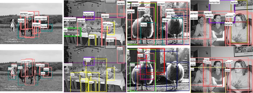
Fig. 7 Example test images. On the top row, we show the top 10 detec- patterns of chair detections that overlap, as maybe common in scenes
tions from the baseline model after standard NMS. On the bottom row, of tables. In the right center, our model exploits co-occurrence cues
we show the top 10 marginal detections from our global model. On the favoring groups of animals. Finally, on the right, our model appears to
left, we see that horse and person detections are better localized by the be exploiting relational cues about sofas and people while enforcing
globally tuned NMS model. In the left center, our model seems to favor mutual exclusion between the bottle and people detections
(2008), Baur et al. (2008). We also learn meaningful mul- on PASCAL. We provide a couple of hypotheses as to why
ticlass spatial layouts—e.g., bottles tend to occur above ta- this is so:
bles. We refer the reader to the captions for additional analy-
sis. Figure 7 shows example multi-class detections from our 1. Contextual layout models are better suited for images
model as compared to the baseline. Our model appears to with multiple objects. The PASCAL dataset is some-
produce better detections by understanding interactions be- what impoverished as far as presence of sufficient inter-
tween objects that spatially overlap, such as people when class and intra-class context is concerned. The PASCAL
riding horses. It also learns how to correctly enforce mu- dataset contains 20 object classes. However, more than
tual exclusion between classes, allowing people and sofas to half the images contain only a single object class with
overlap but not people and bottles. two instances of that object class typically present in
Does context help? Our results suggest that the benefit the image. We agree with the sentiment from Choi et
from using context to improve per-class AP is only marginal al. (2010) that “contextual information is most usefulInt J Comput Vis
when many different object categories are present simul- Table 3 Table comparing the average energy, precision and recall
across different approximation techniques
taneously in an image, with some object instances that
are easy to detect (i.e. large objects) and some instances Av. score Av. prec Av. recall
that are hard to detect (i.e. small objects).” Along similar
lines, Park et al. (2010) suggest that context provides a Greedy 1.174 0.7939 0.4673
stronger improvement for detecting small objects rather TRW-S 1.185 0.771 0.4707
than large objects. We hypothesize that our models may LBP 1.185 0.771 0.4707
similarly exhibit a stronger improvement on datasets con-
taining such variety.
2. Context is more useful for higher-level semantic tasks. is susceptible to getting trapped at non-optimal fix points.
Our baseline local detectors are state-of-the-art models In the TRW approach, the original MAP problem is initially
that have consistently produced competitive results on formulated as an integer program, whose binary constraints
PASCAL in terms of per class AP. We believe that con- are “relaxed” to give a linear program (LP). The TRW algo-
textual reasoning may only provide limited improvement rithm is a variant of Belief Propagation that solves the result-
over highly-tuned local detectors when scored for tasks ing LP and has been shown to be significantly faster for this
such as object detection and localization. This view is problem structure than off-the-shelf LP solvers (Yanover
corroborated by other empirical evaluations of context and Meltzer 2006). The solution given by TRW provides
using tuned local detectors (Divvala et al. 2009) and an upper bound on the solution of our score maximization
(Galleguillos et al. 2008). However, we argue that con- problem. Notably, if the solution to the LP relaxation is in-
text is helpful for higher level semantic inferences such tegral, then the bound is tight and the solution is guaranteed
as scene or action understanding. In the extreme case, to be a global optimum.
given a perfect person and bottle detector, context can- We took the model learned using the approach discussed
not improve detection performance of either class. But in Sect. 5 and ran the 3 approximation techniques: Greedy,
even given such perfect detectors, one still requires a con- LBP and TRW on the test set comprising 4952 images from
textual layout model to recognize “drinking” actions be- PASCAL VOC 2007 dataset. We used the publicly avail-
cause people and bottles must be simultaneously found able software from Meltzer (2006) for LBP and the software
in particular spatial relationships. from MSR (2006) for TRW-S.2 Table 3 compares the ap-
proximation techniques in terms of how well they maximize
Our per-image AP and overall AP scores partially validate the score function, and their accuracy on PASCAL 2007 test
the second hypothesis. Per-image AP scores can be inter- set. For 4942 out of 4952 images (99.8%), Greedy and LBP
preted as a loose proxy for a holistic understanding of a yield identical results. More importantly, for 4832 of the
“scene” since one must reconcile detections across multiple 4952 images (97.6%), all the three schemes produce identi-
classes simultaneously. Under this criteria, our model does cal labels. For these cases, we verified that TRW-S produces
improve AP from 37% to 40%, which is noticeably stronger integer solutions. This means that greedy produces the prov-
than the 1% improvement in overall AP. In subsequent work ably globally optimal solution in almost all images, while
(Desai et al. 2010), we further investigate the effect of con- being two orders of magnitude faster than either approach.
textual layout models on the high-level semantic task of ac- One theoretical explanation for the near-optimal perfor-
tion recognition. We demonstrate that the contextual models mance of the greedy search procedure comes from the study
developed here can be used to increase the accuracy of a of maximizing sub-modular set functions. While such prob-
static-image action classifier by 12%. Notably, this increase lems are NP hard in general, simple greedy heuristics can be
is obtained over a baseline using the exact same state-of- shown to have strong approximation guarantees (Nemhauser
the-art local detectors used here. Hence we believe that our
et al. 1978). If the pairwise weights are all ≤0, then one can
contextual layout model is more rewarding when used for
show that S(X, Y ) from (1) is a submodular set function be-
higher level semantic tasks.
cause it satisfies the diminishing returns property: consider
two sets of instanced windows I1 and I2 , where I1 ⊆ I2 , and
a particular un-instanced window i. The increase in S(X, Y )
7 Analysis of Greedy Inference
due to instancing i must be smaller for I2 because all pair-
wise interactions are negative. This means that greedy infer-
We compare our greedy inference algorithm to two other ap-
ence algorithms enjoy strong theoretical guarantees for con-
proximate inference approaches: Loopy Belief Propagation
textual layout models with solely negative interactions. In
(LBP) and Tree Re-Weighted Belief Propagation (TRW)
practice, we observe that 90% of all the pairwise weights
(Wainwright et al. 2002; Kolmogorov 2006). Although LBP
has been widely used for approximate inference in graphical
2 We
models with cycles, LBP is not guaranteed to converge and also tested QPBO (Rother et al. 2007) which gave similar results.Int J Comput Vis
associated with the model trained on PASCAL 2007 im- then define a CRF over the labels of the segments. This ap-
ages are ≤0, which makes S(X, Y ) close to sub-modular proach has the advantage that unary potentials can now be
and our greedy maximization algorithm theoretically well- defined with object templates, say, centered on the segment.
motivated. However, the initial segmentation must be fairly accurate
and enforces NMS and mutual exclusion without object-
level layout models.
8 Discussion and Related Work To our knowledge, the problem of end-to-end learning
of multi-object detection (i.e. learning NMS) has not been
There has been a wide variety of work in the last few explored. The closest work we know of is that of Blaschko
years on contextual modeling in image parsing (Torralba and Lampert (2008) who use structured regression to pre-
et al. 2004; Sudderth et al. 2005; Hoiem et al. 2008; Gal- dict the bounding box of a single detection within an image.
leguillos et al. 2008; Shotton et al. 2006; He et al. 2004; Both models are trained using images rather an cropped win-
Anguelov et al. 2005). These approaches have typically dows. Both are optimized using the structural SVM formal-
treated the problem as that of finding a joint labeling for ism of Tsochantaridis et al. (2004). However, the underlying
a set of pixels, super-pixels, or image segments and are usu- assumptions and resulting models are quite different. In the
ally formulated as a CRF. Such CRFs for pixel/segment la- regression formalism of Blaschko and Lampert (2008), one
beling use singleton potential features that capture local dis- assumes that each training image contains a single object
tributions of color, textons, or visual words. Pairwise po- instance, and so one cannot leverage information about the
tentials incorporate the labelings of neighboring pixels but layout of multiple object instances, beit from the same class
in contrast to older work on MRFs these pairwise poten- or not. The models may not perform well on images with-
tials may span a very large set of neighboring sites (e.g. out the object because such images are never encountered
Torralba et al. 2004; Tu 2008). Learning such complicated during training. In our model, we can use all bounding-box
potentials is a difficult problem and authors have relied pri- labels from all training images, including those that do not
marily on boosting (Shotton et al. 2006; Torralba et al. 2004; contain any object, to train a model that will predict those
Tu 2008) to do feature selection in a large space of possible very labels.
potential functions.
These approaches are appealing in that they can simul-
taneously produce a segmentation and detection of the ob- 9 Conclusion
jects in a scene. Thus they automatically enforce NMS and
hard mutual exclusion (although as our examples show, this
We have presented a system for multi-class object detection
may not be entirely desirable). However, the discrimina-
with spatial interactions that can be efficiently trained in a
tive power of these methods for detection seems limited.
discriminative, end-to-end manner. This approach is able to
While local image features work for some object classes
fuse the outputs of state of the art template based object de-
(grass, sky etc.), a clear difficulty with the pixel/segment
tectors with information about contextual relations between
labeling approach is that it is hard to build features for
objects. Rather than resorting to post-processing to clean up
objects defined primarily by shape. It still remains to be
detections, our model learns optimal non-max suppression
shown whether such approaches are competitive with scan-
parameters and detection thresholds for each class. The re-
ning window templates on object detection benchmarks.
sulting system outperforms published results on the PAS-
In principle, one could define unary potentials for CRFs
CAL VOC 2007 object detection dataset.
using, say, HOG templates centered on individual pixels.
However, the templates must score well when centered on
Acknowledgements This work was supported by NSF grant
every pixel within a particular segment. Thus templates will 0812428, a gift from Microsoft Research and the UC Lab Fees Re-
tend to be overly-smoothed. Our method is fundamentally search Program.
different in that the output is sparse. A complete object de-
tection is represented by the activation of a single pixel and
so the unary potential can be quite strong. Furthermore, a de- References
tection in our model represses detections corresponding to
small translations while, in the pixel labeling model, exactly Anguelov, D., Taskar, B., Chatalbashev, V., Koller, D., Gupta, D.,
the opposite has to happen. We thus make a tradeoff, moving Heitz, G., & Ng, A. (2005). Discriminative learning of Markov
to more powerful discriminative unary features but sacrific- random fields for segmentation of 3d scan data. In CVPR, II (pp.
169–176).
ing tractable pairwise potentials.
Baur, R., Efros, A. A., & Hebert, M. (2008). Statistics of 3d object lo-
Alternatively, (Galleguillos et al. 2008; Kumar and cations in images (Tech. Rep. CMU-RI-TR-08-43). Robotics In-
Hebert 2005) group pixels into object-sized segments and stitute, Pittsburgh, PA.Int J Comput Vis
Blaschko, M. B., & Lampert, C. H. (2008). Learning to localize objects Workshop on statistical learning in computer vision, ECCV (pp.
with structured output regression. In ECCV (pp. 2–15). Berlin: 17–32).
Springer. Liu, Y., Lin, W., & Hays, J. (2004). Near-regular texture analysis and
Choi, M., Lim, J., Torralba, A., & Willsky, A. (2010). Exploiting hier- manipulation. ACM Transactions on Graphics, 23(3), 368–376.
archical context on a large database of object categories. In IEEE Meltzer, T. (2006). http://www.cs.huji.ac.il/talyam/inference.html.
conference on computer vision and pattern recognition, CVPR MSR (2006). http://research.microsoft.com/en-us/downloads/dad6c31e
Dalal, N., & Triggs, B. (2005). Histograms of oriented gradients for -2c04-471f-b724-ded18bf70fe3/.
human detection. In CVPR I (pp. 886–893). Murphy, K., Torralba, A., & Freeman, W. (2003). Using the forest
Desai, C., Ramanan, D., & Fowlkes, C. (2009). Discriminative models to see the trees: a graphical model relating features, objects and
for multi-class object layout. In IEEE international conference on scenes. NIPS 16.
computer vision. Nemhauser, G., Wolsey, L., & Fisher, M. (1978). An analysis of ap-
Desai, C., Ramanan, D., & Fowlkes, C. (2010). Discriminative models proximations for maximizing submodular set functions. Mathe-
for static human-object interactions. In Workshop on structured matical Programming, 14(1), 265–294.
prediction in computer vision, CVPR. Park, D., Ramanan, D., & Fowlkes, C. (2010). Multiresolution models
Divvala, S., Hoiem, D., Hays, J., & Efros, A. (2009). An empirical for object detection. In ECCV.
study of context in object detection. In CVPR. Rother, C., Kolmogorov, V., Lempitsky, V., & Szummer, M. (2007).
Everingham, M., Van Gool, L., Williams, C. K. I., Winn, J., & Zis- Optimizing binary mrfs via extended roof duality. In CVPR.
serman, A. (2007). The PASCAL visual object classes chal- Rowley, H. A., Baluja, S., & Kanade, T. (1996). Neural network-based
lenge 2007 (VOC2007) results. http://www.pascal-network.org/ face detection. IEEE Transactions on Pattern Analysis and Ma-
challenges/VOC/voc2007/workshop. chine Intelligence, 20, 23–38.
Felzenszwalb, P. (2008). http://people.cs.uchicago.edu/pff/latent.
Shotton, J., Winn, J., Rother, C., & Criminisi, A. (2006). Textonboost:
Felzenszwalb, P., McAllester, D., & Ramanan, D. (2008). A discrimi-
joint appearance, shape and context modeling for multi-class ob-
natively trained, multiscale, deformable part model. In CVPR.
Finley, T., & Joachims, T. (2008). Training structural svms when exact ject recognition and segmentation. Lecture Notes in Computer
inference is intractable. In Proceedings of the 25th international Science, 3951, 1.
conference on machine learning (pp. 304–311). New York: ACM. Sudderth, E., Torralba, A., Freeman, W., & Willsky, A. (2005). Learn-
Franc, V. (2006). http://cmp.felk.cvut.cz/xfrancv/libqp/html. ing hierarchical models of scenes, objects, and parts. In ICCV, II
Galleguillos, C., Rabinovich, A., & Belongie, S. (2008). Object catego- (pp. 1331–1338).
rization using co-occurrence, location and appearance. In CVPR, Teo, C., Smola, A., Vishwanathan, S., & Le, Q. (2007). A scal-
Anchorage, AK. able modular convex solver for regularized risk minimization. In
Hall, E. (1966). The hidden dimension. New York: Anchor Books. SIGKDD. New York: ACM.
He, X., Zemel, R., & Carreira-Perpinan, M. (2004). Multiscale con- Torralba, A., Murphy, K., & Freeman, W. (2004). Contextual models
ditional random fields for image labeling. In CVPR (Vol. 2). Los for object detection using boosted random fields. NIPS.
Alamitos: IEEE Comput. Soc. Tsochantaridis, I., Hofmann, T., Joachims, T., & Altun, Y. (2004). Sup-
Hoiem, D., Efros, A., & Hebert, M. (2008). Putting objects in perspec- port vector machine learning for interdependent and structured
tive. IJCV, 80(1), 3–15. output spaces. In ICML. New York: ACM.
Joachims, T., Finley, T., & Yu, C. (2009). Cutting plane training of Tu, Z. (2008). Auto-context and its application to high-level vision
structural SVMs. Machine Learning, 77(1), 27–59. tasks. In CVPR.
Kolmogorov, V. (2006). Convergent tree-reweighted message pass- Viola, P. A., & Jones, M. J. (2004). Robust real-time face detection.
ing for energy minimization. IEEE Transactions on Pattern IJCV, 57(2), 137–154.
Analysis and Machine Intelligence, 28, 1568–1583. http://doi. Wainwright, M., Jaakkola, T., & Willsky, A. (2002). Map estimation
ieeecomputersociety.org/10.1109/TPAMI.2006.200. via agreement on (hyper)trees: message-passing and linear pro-
Kumar, S., & Hebert, M. (2005). A hierarchical field framework for gramming approaches. IEEE Transactions on Information The-
unified context-based classification. In Tenth IEEE international ory, 51, 3697–3717.
conference on computer vision, ICCV, 2005 (Vol. 2). Yanover, C., & Meltzer, T. Y. W. (2006). Linear programming re-
Leibe, B., Leonardis, A., & Schiele, B. (2004). Combined object cat- laxations and belief propagation—an empirical study. In JMLR
egorization and segmentation with an implicit shape model. In (pp. 1887–1907).You can also read