A Spatially Distributed, Physically-Based Modeling Approach for Estimating Agricultural Nitrate Leaching to Groundwater - MDPI
←
→
Page content transcription
If your browser does not render page correctly, please read the page content below
hydrology
Article
A Spatially Distributed, Physically-Based Modeling Approach
for Estimating Agricultural Nitrate Leaching to Groundwater
Giovanna De Filippis                     , Laura Ercoli and Rudy Rossetto *

                                             Institute of Life Sciences, Scuola Superiore Sant’Anna, Piazza Martiri della Libertà 33, 56127 Pisa, Italy;
                                             giovanna.df1989@libero.it (G.D.F.); l.ercoli@santannapisa.it (L.E.)
                                             * Correspondence: rudy.rossetto@santannapisa.it

                                             Abstract: Nitrogen-nitrate, while being fundamental for crop production, is of particular concern
                                             in the agricultural sector, as it can easily leach to the water table, worsening groundwater quality.
                                             Numerical models and Geographic Information System may support the estimation of nitrate
                                             leaching rates in space and time, to support sustainable agricultural management practices. In this
                                             paper, we present a module for the simulation of the processes involved in the nitrogen cycle in the
                                             unsaturated zone, including nitrate leaching. This module was developed taking steps from the
                                             ANIMO and EPIC model frameworks and coupled to the hydrological models integrated within
                                             the FREEWAT platform. As such, the nitrogen cycle module was then included in the FREEWAT
                                             platform. The developed module and the coupling approach were tested using a simple synthetic
                                             application, where we simulated nitrate leaching through the unsaturated zone for a sunflower crop
                                             irrigated district during a dry year. The results of the simulation allow the estimation of daily nitrate
                                             concentration values at the water table. These spatially distributed values may then be further used
                                             as input concentration in models for simulating solute transport in aquifers.

                                             Keywords: hydrological cycle; nitrogen cycle; hydrological modelling; nitrate leaching; nitrate

                                      groundwater pollution; agricultural water management; groundwater numerical modelling
Citation: De Filippis, G.; Ercoli, L.;
Rossetto, R. A Spatially Distributed,
Physically-Based Modeling Approach
for Estimating Agricultural Nitrate          1. Introduction
Leaching to Groundwater. Hydrology                 Nitrogen-nitrate, while being fundamental for crop production, is of particular concern
2021, 8, 8. https://doi.org/10.3390/         in the agricultural sector, as it can easily leach to the water table, worsening groundwater
hydrology8010008                             quality. Nitrate pollution of water is a major issue worldwide (Mateo-Sagasta et al., 2018;
                                             Wang and Li 2019; Zhang et al., 2019) [1–3]. It originates mostly from the use of inorganic
Received: 4 November 2020                    fertilizers and animal manure in agricultural areas (Liao et al., 2012; Nakagawa et al., 2017;
Accepted: 6 January 2021
                                             Ward et al., 2018; Zhang et al., 2018a) [4–7], and inefficient management of treated/untreated
Published: 11 January 2021
                                             wastewater (Minnig et al., 2018) [8] and solid waste disposal (Wakida and Lerner 2005) [9].
                                             Focusing on groundwater, nitrate contamination is a worldwide problem (Re et al., 2017;
Publisher’s Note: MDPI stays neu-
                                             Zhang et al., 2018b; Ducci et al., 2019; Shukla and Saxena 2019) [10–13]. In Europe, policies
tral with regard to jurisdictional clai-
                                             to reduce NH4 + and NO3 − losses have been in place since nearly 30 years following the
ms in published maps and institutio-
                                             issue of the Nitrates Directive (ND; EC 1991) [14]. The ND objectives have been to reduce
nal affiliations.
                                             water pollution caused or induced by nitrates, and to prevent further pollution. According
                                             to the ND, Member States are asked to identify Nitrate Vulnerable Zones (NVZs), i.e.,
                                             zones with eutrophic water bodies or at risk of eutrophication, with nitrate concentration
Copyright: © 2021 by the authors. Li-        in ground- or surface-water exceeding 50 mg/L (NO3 − regulatory limit for drinking water;
censee MDPI, Basel, Switzerland.             Wild et al., 2018 [15]). Anyway, Wild et al., (2018) [15] argue that it will take several decades
This article is an open access article       to significantly reduce nitrate concentrations in porous aquifers via denitrification, even if
distributed under the terms and con-         future nitrate inputs were considerably reduced.
ditions of the Creative Commons At-                The ND was followed in 2000 by the Water Framework Directive (WFD; EC, 2000 [16]),
tribution (CC BY) license (https://
                                             whose goal is to reach a good chemical and ecological status of water bodies by 2027.
creativecommons.org/licenses/by/
                                             The purposes, objectives, and strategies of the WFD overlap with those of the ND, especially
4.0/).

Hydrology 2021, 8, 8. https://doi.org/10.3390/hydrology8010008                                                   https://www.mdpi.com/journal/hydrology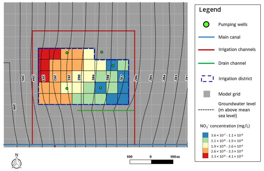
Hydrology 2021, 8, 8                                                                                            2 of 25

                       after the introduction of the Groundwater Directive (EC, 2006 [17]) in 2006. In the attempt
                       to target the objectives of the above-mentioned directives, River Basin Management Plans
                       envisage approaches to assess nitrogen occurrence and to evaluate the effectiveness of
                       measures to reduce nitrogen content in groundwater. Such approaches include monitoring
                       of groundwater quality in NVZs (e.g., Jørgensen et al., 2009 [18]) and evaluation of nitrate
                       leaching through the unsaturated zone and nitrate fate and transport in surface- and
                       ground-water by means of modeling (e.g., Pistocchi et al., 2012; Klement et al., 2018;
                       Husic et al., 2019 [19–21]).
                             The nitrogen cycle (Figure 1) involves physical, chemical, and biological processes
                       which determine an increase or decrease of nitrogen content in the soil and the vadose zone,
                       as well as nitrogen transformation among organic nitrogen (NH2 − ), ammonium (NH4 + )
                       and nitrate (NO3 − ) pools. Three sub-cycles may be distinguished:
                       •    the sub-cycle occurring in the atmosphere;
                       •    the sub-cycle occurring in the unsaturated zone;
                       •    the sub-cycle occurring in the plants, which involves NO3 − uptake by roots.

                       Figure 1. Sketch of the main processes involved in the nitrogen cycle.

                             Sources/sinks contributing to the three nitrogen pools also play relevant roles (e.g., de-
                       riving from surface runoff, fertilizers, etc.). A detailed review on the N cycle in the vadose
                       zone-groundwater system may be found in Xin et al., (2019) [22].
                             Several models are available to simulate watershed/field scale hydrological processes.
                       Some of these models also include methods to simulate the nitrogen cycle in soils and
                       nitrogen leaching, the downward transport of N passing the root zone by percolating water
                       through the unsaturated zone (Golmohammadi et al., 2014 [23]). Appendix A reports the
                       main characteristics of some of these models, in terms of the modeling approach adopted
                       (lumped or spatially distributed), the scale of application, and space and time discretization.
                       Details about the mathematical approach are reported as well, focusing on the hydrological
                       and the nitrogen cycling components only.
                             Most of the codes listed in Appendix A include a hydrological component, except
                       for ANIMO (Groenendijk and Kroes 1999 [24]), which can be coupled to external models
                       (e.g., SIMGRO, Querner and Van Bakel 1989 [25]; SWAP, Van Dam et al., 1997 [26]) for the
                       simulation of water fluxes and moisture contents. In ANIMO, such components are then
                       algebraically summed to get the change in water volume over time, to be used as input
                       in the nitrogen cycling component. In EPIC (Sharpley 1990 [27]), APEX (Williams et al.,
                       2015 [28]) and SWAT (Neitsch et al., 2005 [29]), belonging to the CREAMS (Knisel 1980 [30])
                       family of models, the hydrological component is based on algebraic mass balance equations
                       involving rainfall, runoff, and evapotranspiration and other hydrological processes. On the
                       other hand, other codes (i.e., DAISY, Hansen et al. 1990 [31]); PRZM-3, Suárez 2005 [32];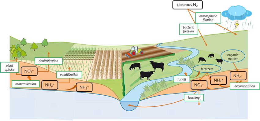
Hydrology 2021, 8, 8                                                                                                              3 of 25

                                    and NTT-Watershed, Heng and Nikolaidis 1998 [33]) solve the Richards’ equation for soil
                                    water dynamics in the unsaturated zone.
                                         Regarding the nitrogen cycling component, all the codes reported in Appendix A
                                    integrate equations for the simulation of the processes involved in the nitrogen cycle.
                                    DAISY and PRZM-3 simulate NH2 − mineralization in a very detailed way, including
                                    different NH2 − sub-pools and resulting in large-parameterized models. EPIC, APEX,
                                    and SWAT use soil-dependent decay coefficients for the simulation of nitrogen leaching
                                    through the unsaturated zone, while ANIMO, DAISY, PRZM-3, and NTT-Watershed solve
                                    1D advection-dispersion solute transport equations in the unsaturated zone.
                                         Nitrate leaching research grew in the scientific community in the last decades (Padilla et al.,
                                    2018 [34]), focusing also on modeling methodologies (Canter 2019 [35]). Indeed, assessing
                                    nitrogen transport and turnover in the unsaturated zone and in groundwater is an expen-
                                    sive and complex task to be run at field scale (Sutton et al., 2011 [36]). At the same time,
                                    advances in distributed modeling efforts that incorporate spatial distribution of nitrogen
                                    inputs, soil and aquifer characteristics, land use data, and farming practices are promising
                                    (Xu et al., 2013; Ransom et al., 2017 [37,38]). While several modeling studies focused
                                    on simulating soil nitrogen balance or groundwater nitrogen transport independently
                                    (Wriedt 2004 [39]; Epelde et al., 2016 [40]), there is a clear trend to combine unsaturated
                                    zone and groundwater flow models for the simulation of nitrogen dynamics [41–43].
                                         As such, in the following sections, we present a new modeling approach in order to
                                    compute nitrate leaching to the water table based on (a) the development of a numerical
                                    module for the simulation of the nitrogen cycle in the unsaturated zone, (b) the integration
                                    of such module in the Geographic Information System (GIS)-integrated FREEWAT platform
                                    (Foglia et al. 2018 [44]). The module was developed taking steps from the ANIMO and
                                    EPIC lumped models. Once developed, the module was then coupled to physically-based,
                                    spatially distributed codes for the simulation of unsaturated zone flow and agricultural
                                    water management and, finally, included into the GIS-integrated FREEWAT platform.

                                    2. Materials and Methods
                                    2.1. Overview of the Nitrogen Cycle Module
                                          The nitrogen cycle module here developed allows to simulate the processes determining
                                    an increase or decrease of nitrogen content in the unsaturated zone, as well as nitrogen
                                    transformation among the NH2 − , NH4 + , and NO3 − pools (Figure 1). The module developed
                                    is based on the conceptualization of the ANIMO model [24]. ANIMO simulates the nitrogen
                                    budget for the three pools, by solving a partial differential equation for each of them (Table 1).
                                    All terms and symbols listed in Table 1 are detailed in Appendices B and C. Figure 2 reports a
                                    sketch of all the processes related to nitrogen mass flux in the unsaturated zone, occurring
                                    within a grid cell. By solving the equations reported in Table 1, the variation of nitrogen
                                    concentration for each pool in time and space, in the unsaturated zone, is calculated.

      Table 1. Partial differential equations solved by the ANIMO model for the three nitrogen pools (modified after Groenendijk
      and Kroes 1999 [24]).

                                                     Vertical           Lateral Outflow   Crop Uptake    Decomposition Production
   Nitrogen Pool       Conservation Term
                                                    Flow Term                Term            Term           Term          Term
        NH2 −              ∂(θ (t)c NH2 (t))
                                   ∂t
                                                =   −
                                                        ∂Js,NH2 (t,z)
                                                             ∂z
                                                                          − R x,NH2 (t)                  − Rd,NH2 (t)     + R p,NH2 (t)
                          ∂(θ (t)c NH4 (t))
                                            +           ∂Js,NH4 (t,z)
        NH4 +                    ∂t
                                ∂Xe,NH4 (t)
                                                =   −                     − R x,NH4 (t)   − Ru,NH4 (t)   − Rd,NH4 (t)     + R p,NH4 (t)
                                                             ∂z
                           ρd       ∂t
        NO3 −              ∂(θ (t)c NO3 (t))
                                   ∂t
                                                =   −
                                                        ∂Js,NO3 (t,z)
                                                             ∂z
                                                                          − R x,NO3 (t)   − Ru,NO3 (t)   − Rd,NO3 (t)     + R p,NO3 (t)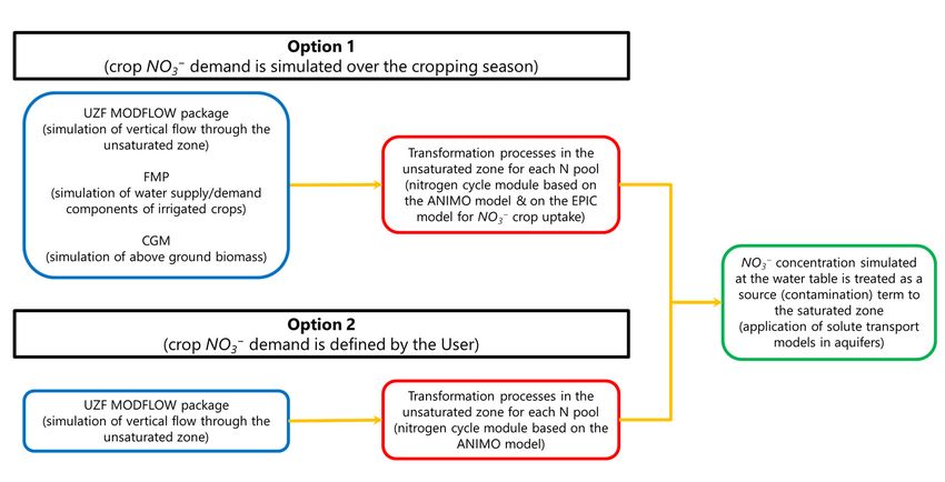
Hydrology 2021, 8, 8                                                                                                   4 of 25

                       Figure 2. Sketch of all the processes related to nitrogen mass flux in the unsaturated zone, occurring
                       within a grid cell.

                             The following terms appear in the equations presented in Table 1:
                       •     a conservation term, which expresses the variation of nitrogen concentration in time;
                                                                                                       ∂X      (t)
                       •     the conservation term for NH4+ includes also sorption by soil (ρd e,NH4  ∂t   );
                       •     a vertical, unidimensional transport term, which is driven by unsaturated zone flow;
                       •     a term related to lateral movement of nitrogen in the unsaturated zone (lateral outflow
                             term). However, in our approach, we assume that vertical transport of nitrogen is the
                             predominant process. As such, lateral movement of nitrogen is not simulated;
                       •     a crop uptake term for NO3 − and NH4 + . Such term is estimated for NO3 − only,
                             adopting the EPIC model approach (Sharpley 1990) [27], taking into account the
                             phenological phases of crops. We assume, indeed, that NO3 − is the predominant form
                             of available nitrogen uptaken by roots (Nadelhoffer et al. 1984; Xu et al. 2012) [45,46];
                       •     a decomposition term, i.e., mineralization for NH2 − , nitrification for NH4 + , denitrifi-
                             cation for NO3 − ;
                       •     a production/loss term, which includes source/sink terms for each pool and the
                             decomposition term from the above pool (i.e., NH2 − represents the pool above NH4 + ,
                             and NH4 + represents the pool above NO3 − ).
                             The relation among the three pools is guaranteed through the decomposition mechanisms:
                       (a)   mineralization of organic nitrogen represents a sink term for the NH2 − pool and
                             a source term for the NH4 + pool. As such, this is subtracted in the decomposition
                             term for NH2 − (R_(d,NH2) in Table 1) and summed as production term for NH4 +
                             (R_(p,NH4 ) in Table 1);
                       (b)   nitrification of ammonium represents a sink term for the NH4 + pool and a source
                             term for the NO3 − pool. As such, this is subtracted in the decomposition term for
                             NH4 + (R_(d,NH4 ) in Table 1) and summed as production term for NO3 − (R_(p,NO3 )
                             in Table 1).
                             The equations reported in Table 1 are solved one by one, in the order presented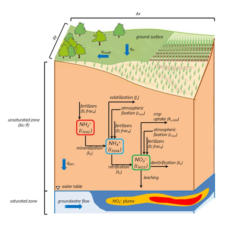
Hydrology 2021, 8, 8                                                                                                              5 of 25

                                      above. Each of them can be rewritten as (subscripts NH2 , NH4 and NO3 will be omitted in
                                      the following):

                                     dc(t)  q (t)[crain (t) + c(t0 )]    q perc (t)c(t)
          [θ (t0 ) + ϕ∆t + ρd Kd ]         = in                       −                 − Kup c(t) − λ1 θ (t)c(t) + R p − ϕc(t)      (1)
                                      dt              ∆z                ∆z ∗ ∆x ∗ ∆y

                                          By solving Equation (1), concentration in time (c(t)) for each pool is calculated in the
                                      unsaturated zone at the time t.
                                          We decided to take steps from the ANIMO, among the models listed in the Appendix A,
                                      because we considered it a good compromise with respect to the following aspects:
                                      -    the mathematical approach adopted, based on the mass conservation and the solution
                                           of transport Equation (1);
                                      -    the mathematical approach adopted is relatively frugal, in the sense that it requires
                                           few input parameters;
                                      -     the integration between Equation (1) and the unsaturated zone flow term calculated
                                           by means of distributed models integrated within the FREEWAT platform was pretty
                                           straightforward with respect to the space and time dimension of the involved processes.

                                      2.2. Overview of the FREEWAT Platform
                                            FREEWAT [47] is a free and open source platform integrated in a GIS framework for
                                      water resource management, with a specific focus on groundwater, initially developed within
                                      the HORIZON 2020 FREEWAT project (FREE and open source software tools for WATer
                                      resource management; www.freewat.eu; [48]), a follow up of the SID & GRID platform [49].
                                            FREEWAT is conceived as a QGIS [50] plugin, which integrates free and open source
                                      software tools for pre- and post-processing of spatial data, and numerical codes for the
                                      simulation of the hydrological cycle. On one side, GIS and spatial database management ap-
                                      plications [51] are exploited for spatial data storage, visualization and analysis. Physically-
                                      based and spatially distributed numerical models (i.e., MODFLOW, Harbaugh 2005 [52],
                                      and MODFLOW-related models) integrated within the FREEWAT platform allow to simu-
                                      late several processes involved in the hydrological cycle (e.g., groundwater flow, density-
                                      dependent flow, conjunctive use of ground- and surface-water, solute transport, sensitivity
                                      analysis and model calibration). Dedicated tools for pre-processing of field data [53,54] and
                                      for post-processing of models’ results are integrated as well. FREEWAT was applied to date
                                      to a variety of case studies [55]. The present work may be considered as a continuation of
                                      the research activities performed to better describe agricultural water use in hydrological
                                      modelling. In particular, the Farm Process (FMP; embedded in the USGS’s MODFLOW
                                      One-Water Hydrologic Model [56]) coupled to a Crop Growth Model (CGM [57]) for sim-
                                      ulating crop yield based on solar radiation and biomass accumulation was previously
                                      integrated within the FREEWAT platform.

                                      2.3. Coupling the Nitrogen Cycle and the Hydrological One
                                           The nitrogen cycle module was coupled to the unsaturated flow process, in order to
                                      simulate advective transport of nitrogen compounds in the downward direction, across the
                                      unsaturated zone. According to the ANIMO approach, the nitrogen concentration in the
                                      outflowing water, moving from one unsaturated zone layer to another, is equal to the calcu-
                                      lated nitrogen concentration within the ith unsaturated zone layer [24]. In our approach, by
                                      activating the Unsaturated Zone Flow (UZF) MODFLOW package [58] in a groundwater
                                      flow model based on MODFLOW-2005 [52], we simulate a fraction of the total nitrogen
                                      mass within the unsaturated zone that reaches the water table. The nitrogen mass flow is
                                      driven by vertical water flow through the unsaturated zone. The UZF solves a kinematic
                                      wave approximation of the Richards’ equation to simulate vertical flow and storage through
                                      the unsaturated zone [58]. Conversely from most of the lumped available codes simulating
                                      the nitrogen cycle (e.g., ANIMO and EPIC), the codes integrated in the FREEWAT platform
                                      for the simulation of the unsaturated zone are spatially distributed. Hence, the partial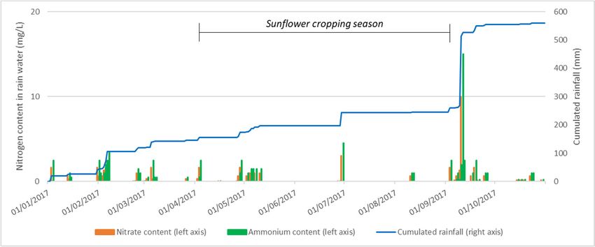
Hydrology 2021, 8, 8                                                                                                         6 of 25

                                 differential equations are solved to get the involved variables (e.g., hydraulic head and
                                 solute concentration) also in a discretized space.
                                      The coupling approach includes agricultural water management processes for the
                                 representation of inorganic nitrogen uptake by plants’ roots. To this scope, the coupled
                                 FMP-CGM approach developed in FREEWAT for agricultural water management and
                                 crop yield simulation is adopted: in the nitrogen cycle module, input and output of an
                                 FMP-CGM scenario are used to calculate NO3 − crop demand, as conceptualized in the
                                 EPIC model [27]. Specifically, NO3 − crop demand over the different phases of the cropping
                                 season is calculated in EPIC as the difference between the NO3 − crop content, which is the
                                 nitrogen amount in plant biomass, and the NO3 − availability in the soil. Crop transpiration
                                 fluxes simulated by FMP and cumulated biomass calculated by CGM are involved in the
                                 computation of these two variables.
                                      All of the processes involved in the nitrogen cycle were simulated in the unsaturated
                                 zone layer at each cell of a finite-difference grid. This allows to obtain the spatial variation
                                 of nitrogen concentration for each nitrogen pool in the unsaturated zone.
                                      The coupling approach just presented is drawn in Figure 3. The left side of Figure 3
                                 (blue boxes) reports the codes that must be run before running the nitrogen cycle module.
                                 Two options may occur:
                                 -    if crop NO3 − demand is simulated over the cropping season (Option 1), the following
                                      is needed:
                                      •     running a MODFLOW-2005 model, including the UZF Package, to simulate
                                            water flow through the unsaturated zone. This is needed for the calculation of
                                            the thickness of the unsaturated zone, the water content, the runoff rate and the
                                            leaching rate in space and time;
                                      •     running an FMP-CGM scenario. This is needed for the calculation of crop tran-
                                            spiration flux and cumulated above-ground biomass;
                                 -    if crop NO3 − demand is not simulated, but the User inputs crop NO3 − require-
                                      ment parameters over the cropping season (Option 2). In such case, only running a
                                      MODFLOW-2005 model, including the UZF Package, is needed to simulate water
                                      flow through the unsaturated zone as above-mentioned.

      Figure 3. Overview of the coupling approach designed to integrate the nitrogen cycle module within the FREEWAT platform.

     1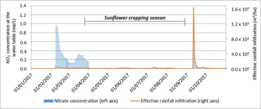
Hydrology 2021, 8, 8                                                                                                      7 of 25

                            The center of Figure 3 (red boxes) reports the simulated nitrogen cycle processes:
                       -    if Option 1 occurs, all of the processes involved in the nitrogen cycle are simulated
                            taking steps from the ANIMO model approach, except for the NO3 − crop uptake
                            process, which is simulated through a sub-routine based on the EPIC model approach;
                       -    if Option 2 occurs, all the processes involved in the nitrogen cycle are simulated
                            taking steps from the ANIMO model approach. In such case, the sub-routine based
                            on the EPIC model approach is not executed, and the NO3 − crop uptake process is
                            simulated by comparing the crop NO3 − requirement defined by the User with the
                            NO3 − availability in the unsaturated zone.
                             In both options, input/output parameters involved in the execution of the UZF,
                       FMP, and CGM components are exploited to run the nitrogen cycle module (i.e., to solve
                       Equation (1)). As a result, the NO3 − concentration at the water table is determined at
                       each cell and for each stress period. This concentration can then be treated as a potential
                       contaminant source term to the saturated zone in solute transport modelling of aquifers
                       (e.g., through the application of the MT3DMS code [59]), as indicated in the green box on
                       the right side of Figure 3.

                       2.4. Model Testing Using a Synthetic Case Study
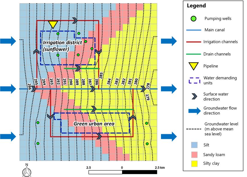
                            The coupling approach discussed in this paper was tested using a synthetic case study
                       presented in Rossetto et al. (2019) [57]. There, the FMP-CGM methodology was applied
                       for simulating daily conjunctive use of ground- and surface-water for the irrigation of
                       sunflower. Sunflower yield at harvest was estimated based on crop phenology, climate
                       conditions, and water availability. Here, we coupled the nitrogen module to that case study
                       in order to exploit settings and results of the above-mentioned model. We focused our
                       attention on the sunflower irrigated Water Demand Unit. Model settings are described in
                       the following and reported in Figure 4.

                       Figure 4. Model settings for the synthetic case study application. The dotted lines refer to the simulated
                       groundwater level on 1 April 2017 (modified after Rossetto et al., 2019) [57].
Hydrology 2021, 8, 8 8 of 25
The whole model extends over an area of 115 km2 and it is discretized by means of
square cells with 500 m of side length. For the calculation of sunflower water root uptake, root
depth values and capillary fringe for the three soil types (silt, silty clay, and sandy loam) are
assigned. Groundwater is pumped from a sandy aquifer represented through a homogeneous,
MODFLOW convertible model layer with variable thickness. Groundwater is delivered to
the irrigation district by six pumping wells. Groundwater flow occurs from west to east.
The model was run in transient conditions between 1 January and 31 October 2017, with
daily stress periods. Irrigation of sunflower was simulated following sunflower seeding on
1 April and up to 31 August 2017 (when the crop was harvested). During the crop growth the
cumulated rainfall depth was 99.8 mm, mainly distributed over four rainfall events occurring
between April and August. Model results showed that sunflower water demand is primarily
met by precipitation and root uptake, and secondly by irrigation water. Further information
on the case study may be found in Rossetto et al., (2019) [57].
The nitrogen cycle module was applied to the present case study to simulate daily
nitrate leaching to the water table.
In order to solve Equation (1) for the NH2 − , NH4 + and NO3 − pools, initial concentra-
tion for each nitrogen compound was defined according to the total content of nitrogen
in the soil and to the soil type. The following equations were used for such estimation
(Masoni 2010) [60]:
c NH − (t0 = 0) = 0.95 ρ a NT (2)
2
c NH + (t0 = 0) = 0.04 ρ a NT (3)
4
c NO− (t0 = 0) = 0.01 ρ a NT (4)
3
For the application of Equations (2)–(4) we assumed: NT = 10−3 kg/kg (Masoni 2010) [60],
ρa = 1360 kg/m3 for silt, ρa = 1440 kg/m3 for sandy loam, and ρa = 1200 kg/m3 for silty
clay (Yu et al., 1993) [61].
This resulted in an initial concentration in the irrigation district ranging between
1140 mg/L and 1368 mg/L for NH2 − , between 48 mg/L and 58 mg/L for NH4 + , and be-
tween 12 mg/L and 14 mg/L for NO3 − .
Nitrogen concentration in rain water varies according to the intensity of precipitation.
Figure 5 reports the content of NH4 + and NO3 − in rain water over the simulation (Eriks-
son 1952) [62], compared to the cumulated rainfall. Peak values of the nitrogen content in
rain water were input when rainfall events occurred.
Figure 5. Variation of nitrogen content in rain water and cumulated rainfall over the simulation period.
Decomposition processes for each nitrogen pool were simulated assuming that the
first order decay rate constant (λ1 ) was equal to 0.01 day−1 (Groot et al., 2012) [63]. As a con-
sequence, here we assumed that mineralization, nitrification, and denitrification contribute
to a 1% daily decrease of NH2 − , NH4 + and NO3 − content, respectively.
Moreover, NH4 + volatilization and sorption were simulated. We assumed that the
volatilization fraction (fv ) was equal to 0.001. For simulating sorption, we used the same val-Hydrology 2021, 8, 8 9 of 25
ues as the apparent density for ρd , and the following values for the Cation Exchange Capac-
ity (CEC): 148 meq/kg for silt, 110 meq/kg for sandy loam, 146 meq/kg for silty clay [64].
For simulating nitrate uptake by sunflower roots over the cropping season, we ex-
ploited results from the FMP-CGM model presented in [57]. As such, we adopted the
approach based on the EPIC conceptualization, by setting the following for sunflower [27]:
bn1 = 0.05, bn2 = 0.023, bn3 = 0.0146, PHU = 1600.
In order to define the N fertilizer rate to be applied for achieving the simulated
sunflower yield, we applied a conventional N balance approach, as
Nf = Nd − (Nr + Ni + Nm ) + (Nl + Nv + Nde ) ± Np (5)
where Nf is N fertilizer rate, Nd is crop N demand, Nr is N supplied by rainfall, Ni is N
supplied by irrigation, Nm is mineralized N from soil organic matter, Nl is N loss from
leaching, Nv is N loss from volatilization, Nde is N loss from denitrification, and Np is N
released (positive) or taken from soil (negative) for residue decomposition of the preceding
wheat crop. All terms in the equation are expressed as kg N ha−1 .
Sunflower N demand (Nd) for 5 Mg ha−1 grain yield with 3.3% grain N concentration,
harvest index 0.4 and 1.0% residue N concentration is 240 kg N ha−1. Nitrogen supply from
rainfall and irrigation was 2 and 23.5 kg ha−1, respectively, and from soil organic matter
mineralization was 36.8 kg ha−1 from the silt soil and 43.6 kg ha−1 from the sandy-loam soil.
Nitrogen loss from leaching, denitrification, and volatilization were assumed to be negligible.
Indeed, the amount of irrigation was calculated to avoid percolation and since soils are well
drained, they do not offer favorable anaerobic conditions for denitrification. Finally, we assume
negligible NH3 emissions occur with soil incorporation of urea (Rochette et al., 2013) [65].
Consequently, Nf was estimated 185.6 kg N ha−1 for the silt soil and 178.8 kg N ha−1
for the sandy-loam soil. We then applied the following values for the dose of fertilization:
D = 1.856 × 10⁻² kg/m2 for silt and D = 1.788 × 10⁻² kg/m2 for sandy loam. Such values
were assigned the day before the beginning of the sunflower cropping season (31 March),
and the whole amounts were assigned to the NH2 − pool only ( f rac NH2 = 1; f rac NH4 = 0;
f rac NO3 = 0). Table 2 presents the dataset used.
Table 2. Values set for the input parameters in the case study.
Parameter Units of Measurements Value
NT kg/kg 10−3
1360 (silt)
ρa and ρd kg/m3 1440 (sandy loam)
1200 (silty clay)
λ1 day−1 10−2
fv 10−3
148 (silt)
CEC meq/kg 110 (sandy loam)
146 (silty clay)
bn1 0.05
bn2 0.023
bn3 0.0146
PHU 1600
1.856 × 10⁻² (silt)
D kg/m2
1.788 × 10⁻² (sandy loam)
f rac NH2 1
f rac NH4 0
f rac NO3 0Hydrology 2021, 8, 8 10 of 25
3. Results and Discussion
The simulation performed allowed us to estimate daily concentration values of NO3 −
arriving at the water table. Figure 6 presents the daily values of NO3 − concentration
simulated at the water table over the simulation period, with respect to the simulated
effective rainfall infiltration through the unsaturated zone. We can notice that leaching
occurs before the crop seeding (between early February and early April 2017) and then
around mid-September 2017. These leaching events are mostly related to rainfall events
concentrated in those periods (Figures 5 and 6). On February–April 2017, daily NO3 −
concentration reaching the water table may reach values up to about 1 mg/L, while values
up to about 1.3 mg/L were simulated on mid-September 2017. From the results of the sim-
ulation, we explain the relatively high concentration arriving at the water table following
rainfall events before the crop season due to the absence of the crop uptake term—similarly,
such concentration increases at the end of the crop season, after crop harvesting (that is,
no more crop nitrogen uptake). On the other hand, during the sunflower cropping season
(April to end of August), the daily NO3 − concentration values at the water table have very
low values (in the order of 10−3 mg/L), as a result of the drought period simulated and of
crop uptake (Figure 6). Our results show a potential risk of NO3 − leaching during the win-
ter wet season. Moreover, substantial NO3 − leaching losses may be due to high-intensity
rainfalls, such as the one occurred in September 2017. Unfortunately, data coming from
experimental activities about daily concentration of NO3 − arriving at the water table are
not published yet—and because of this it was not possible to validate the simulated values.
Figure 6. Daily simulated NO3 − concentration arriving at the water table and the effective rainfall
infiltration over the simulation period.
The time-varying simulated data in Figure 6 refers to one single point in space. Figure 7
shows the spatial distribution of NO3 − concentrations arriving at the water table. At the
selected time nitrogen crop demand is high. The available nitrogen is uptaken through the
roots, and, as result of the simulation, we have very low values of NO3 − concentrations
arriving at the water table. These concentration values may then be used to define the time
and spatially variant source term for simulation of nitrate transport in aquifers (e.g., using
the MT3DMS code [59]).
2Hydrology 2021, 8, 8 11 of 25
Figure 7. Example of simulated spatially distributed values of nitrate concentrations arriving at the
water table (focus over the irrigation district).
The coupling approach presented holds the following limitations:
- the unsaturated zone is discretized in only one layer. It is then considered as a unique
layer extending from the ground surface to the water table. This representation may
not be suitable in case of non-homogeneous soil sediments, with different physical
and chemical properties. Furthermore, NO3 − uptake at different depths according to
the root distribution in the vertical domain may not be adequately reproduced;
- purely advective transport of nitrogen through the unsaturated zone is simulated
(dispersion is neglected);
- the biological fixation process is not simulated. This can lead to underestimation of
mineral nitrogen available in the soil;
- volatilization of NH4 + is taken into account through a volatilization coefficient (fv )
only, which is difficult to quantify;
- NH4 + uptake by plants’ roots is not simulated (we assume, indeed, that NO3 − is the
predominant form of available nitrogen uptaken by roots);
- taking steps from the UZF MODFLOW package approach, we assume that vertical
movement of nitrogen is the predominant process. As such, lateral movement of
nitrogen across neighboring cells is not simulated;
- when the thickness of the unsaturated zone varies, according to water level fluctua-
tions, the mass of nitrogen stored in the soil is simply redistributed over the whole
unsaturated thickness.
Due to the number of required parameters, reduced compared to other simulation
methods, but still very large, we were only able to validate this approach by means of a
synthetic case study. Validation by means of real data is however needed, i.e., to verify
in a real environment the processes that lead to the low concentration values in Figure 7.
Indeed, coupling the nitrogen to the hydrological cycle means, when coming to model
validation, to get data on the hydrology, the crop growth and nitrate cycle at the same
time, which is more than 50 parameter’s values required (see Appendix B for details) with
related uncertainties evaluation. In this sense, experimental trials ranging from lysimeters
to field scale pilot (as in [66–68]), even with high-resolution lysimeters [69] may allow to
get the required data. Dedicated field scale experiments, where longer flowpaths through
the unsaturated zone may be taken into account, using also state-of-the art ground and
remote sensors will allow to complete the validation
3 of the presented approach.Hydrology 2021, 8, 8 12 of 25
4. Conclusions
Agriculture-related activities very often cause leaching of high levels of nutrients in
the soil and the connected aquatic ecosystems, including groundwater. Among nutrients,
nitrate is of particular concern, as it is conservative and it may rapidly leach to the water
table, causing high, or even exceeding, according to ongoing regulations, concentrations in
aquifers and, consequently, potential negative effects on the environment and even human
health, in case groundwater is used for drinking purposes.
In this paper, we described the development of a nitrogen module for the simulation
of the nitrogen cycle in the unsaturated zone and the nitrate leaching process. The de-
veloped module takes steps from the mathematical framework of the ANIMO model,
which solves a mass conservation and transport equation for dissolved organic nitrogen,
nitrate, and ammonium to quantify the relation between fertilization, soil management and
nutrients leaching occurring over time in a vertical soil column. The simulation of nitrate
crop demand and root uptake, instead, is based on the more robust conceptualization of
the EPIC model, which accounts for the different phases of the cropping season to calculate
crop nitrate content and need.
We integrated the developed nitrogen cycle module within the GIS-based FREEWAT
platform, in order to couple it with the spatially distributed codes (e.g., MODFLOW)
for the simulation of unsaturated zone and groundwater flow processes. Thanks to the
integration, we exploited inputs and outputs from the hydrological models to test the
developed modules for simulating the processes involved in the nitrogen cycle. To do so,
the nitrogen cycle module was developed to run at each cell and for the same stress periods
of a MODFLOW model previously set. More specifically, the developed module exploits
results from the UZF MODFLOW package for getting the water content and thickness of
the unsaturated zone, and infiltration and runoff rates generated during rainfall events.
Moreover, results from an agricultural water management scenario based on the application
of FMP-CGM are used to determine the nitrate demand by crops over the growing season.
The coupling approach just summarized guarantees the possibility to implement
nitrogen cycle scenarios requiring relatively few inputs. The simulate daily nitrate concen-
tration at the water table distributed in space is the main relevant output derived from this
simulation approach.
The presented effort is an initial stage of research in producing usable numerical tools
for improving nitrogen management in agricultural fields. Further development of the code
may include, among the others, the integration of lateral movement of nitrogen between
neighboring cells, and the simulation of root uptake with a finer vertical discretization
based on root depth and distribution.
Author Contributions: Conceptualization, G.D.F. and R.R.; methodology, G.D.F. and R.R.; software,
G.D.F.; validation, G.D.F., L.E. and R.R.; formal analysis, G.D.F. and R.R.; resources, R.R.; data
curation, G.D.F. and L.E.; writing—original draft preparation, G.D.F. and R.R.; writing—review and
editing, G.D.F., L.E. and R.R.; visualization, G.D.F. supervision, R.R.; project administration, R.R.;
funding acquisition, R.R. All authors have read and agreed to the published version of the manuscript.
Funding: This paper presents part of the results achieved within the framework of the SMAQua
(SMart ICT tools per l’utilizzo efficiente dell’AcQua; www.freewat.eu/smaqua-project) project, co-
financed by Regione Toscana, ASA S.p.A. and ERM Italia S.p.A and Scuola Superiore Sant’Anna
(2018–2020; POR FSE 2014–2020 CUP J56J17000570004) within the programme RING—Regione Toscana,
imprese e Sant’Anna: percorsi di sviluppo per giovani innovatori.
Acknowledgments: We wish to thank three anonymous reviewers and one academic editor at
Hydrology for their comments and suggestions which helped in improving the quality of the paper.
Giovanna De Filippis (now AECOM URS Italia S.p.A., Milano, Italy) performed the research activities
as post-doc during the SMAQua project at the Institute of Life Sciences (Scuola Superiore Sant’Anna,
Pisa, Italy).
Conflicts of Interest: The authors declare no conflict of interest.Hydrology 2021, 8, 8 13 of 25
Appendix A
Table A1. Review of existing codes for the simulation of the nitrogen cycle in soils and nitrogen leaching through the unsaturated zone.
Modelling Approach
Spatial Hydrological Nitrogen Cycling
Code References (lumped/Spatially Scale of Application Time Discretization
Discretization Component Component
Distributed)
Organic/inorganic
transformations based on
first-order decay functions
involving soil water content,
Watershed divided Based on algebraic
temperature, mineral
into smaller mass balance
nitrogen availability, and the
EPIC Sharpley 1990 Lumped Field scale drainage areas; Daily equation involving
amount of soluble carbon
Soil profile divided rainfall, runoff and
associated with soil
into layers evapotranspiration
organic matter;
Nitrogen leaching estimated
by an exponential decay
weighting function
Organic/inorganic
transformations based on
first-order decay functions
Watershed divided involving soil water content,
Based on algebraic
into hydrologically temperature, mineral
mass balance
Farms and small connected nitrogen availability, and the
APEX Williams et al., 2015 Lumped Daily equation involving
watersheds scales landscape units; amount of soluble carbon
rainfall, runoff and
Soil profile divided associated with soil
evapotranspiration
into layers organic matter;
Nitrogen leaching estimated
by an exponential decay
weighting functionHydrology 2021, 8, 8 14 of 25
Table A1. Cont.
Modelling Approach
Spatial Hydrological Nitrogen Cycling
Code References (lumped/Spatially Scale of Application Time Discretization
Discretization Component Component
Distributed)
Organic/inorganic
transformations based on
Watershed divided Based on algebraic algebraic equations
into Hydrologic mass balance involving soil water content,
SWAT Neitsch et al., 2002 Lumped Watershed scale Response Units; Daily equation involving temperature, and soil
Soil profile divided rainfall, runoff and organic matter availability;
into layers evapotranspiration Nitrogen leaching estimated
by multiplying the leaching
rate by a decay coefficient
Water fluxes and Conservation and transport
moisture contents are equation solved for
Watershed divided computed by dissolved organic nitrogen,
Groenendijk and Field and into sub-regions; external models, and nitrate and ammonium;
ANIMO Lumped Any (not sub-daily)
Kroes 1999 regional scales Soil profile divided then algebraically Nitrogen leaching estimated
into layers summed to get the by means of a 1D transport
change in water equation in the
volume over time unsaturated zone
The organic nitrogen pool is
represented in a very
detailed way, with
further sub-pools;
Based on Richards’ Inorganic transformations
Watershed divided
equation for soil based on algebraic equations
Field and into sub-regions;
DAISY Hansen et al., 1990 Lumped Daily water dynamics, and involving soil water content,
regional scales Soil profile divided
on Darcy’s law for temperature, and
into layers
vertical flow rate carbon availability;
Nitrogen leaching estimated
by means of a 1D transport
equation in the
unsaturated zoneHydrology 2021, 8, 8 15 of 25
Table A1. Cont.
Modelling Approach
Spatial Hydrological Nitrogen Cycling
Code References (lumped/Spatially Scale of Application Time Discretization
Discretization Component Component
Distributed)
Evapotranspiration
from the root zone
estimated directly
from pan The organic nitrogen pool is
evaporation data, or represented in a very
based on an detailed way, with
Watershed divided empirical formula; further sub-pools;
into sub-regions; Water leaching Inorganic transformations
Field and Soil profile divided through the root based on first-order kinetics
PRZM-3 Suárez 2005 Lumped Daily
regional scales into two layers (root zone simulated using involving soil water content
zone and generalized soil and temperature;
unsaturated zone) parameters, and Nitrogen leaching estimated
saturation by means of a 1D transport
water content; equation in the
Flow in the unsaturated zone
unsaturated zone
simulated by
Richards’ equation
Green-Ampt
Organic/inorganic
equation used to
transformations based on
determine the
Watershed first-order kinetics involving
infiltration capacity
discretized into soil water content
NTT- Heng and of the soil;
Spatially distributed Watershed scale square cells; Any and temperature;
Watershed Nikolaidis 1998 Richards’ equation
Soil profile divided Nitrogen leaching estimated
used to simulate the
into layers by means of a 1D transport
vertical movement of
equation in the
water in the
unsaturated zone
unsaturated zoneHydrology 2021, 8, 8 16 of 25
Appendix B
Table A2. Parameters involved in the equations of the nitrogen cycle module.
Symbol Description Dimensions Note
Time instant referring to the beginning of Retrieved from the groundwater flow
t0 [T]
a stress period model setup
Time instant referring to the end of a Retrieved from the groundwater flow
t [T]
stress period model setup
Cartesian coordinate along the
z [L]
vertical direction
∂
∂t
Time derivative [T−1 ]
Spatial derivative along the
∂ [L−1 ]
∂z vertical direction
Retrieved from the groundwater flow
∆t Length of the stress period [T]
model setup
Retrieved from the groundwater flow
∆x Column width of the grid cell [L]
model setup
Retrieved from the groundwater flow
∆y Row width of the grid cell [L]
model setup
∆z Thickness of the unsaturated zone [L] Estimated by UZF package
Retrieved from the groundwater flow
sp Stress period number
model setup
Retrieved from the groundwater flow
Nsp Number of stress periods
model setup
AW Plant available water User-defined
Estimated by CGM and converted
B Cumulated biomass [M/L2 ]
into kg/ha
Crop parameter expressing NO3 −
bn1 User-defined
concentration in the crop at emergence
Crop parameter expressing NO3 −
bn2 concentration in the crop at emergence at User-defined
0.5 maturity
Crop parameter expressing NO3 −
bn3 concentration in the crop at emergence User-defined
at maturity
CEC Cation Exchange Capacity of the soil [meq/M] User-defined
c NH2 Concentration of NH2 − [M/L3 ] Derived variable
c NH4 Concentration of NH4 + [M/L3 ] Derived variable
c NO3 Concentration of NO3 − [M/L3 ] Derived variable
c Nitrogen concentration [M/L3 ] Derived variable
Initial nitrogen concentration
c0 [M/L3 ] Derived variable
(initial condition)
crain Nitrogen concentration in the rain water [M/L3 ] User-defined
c NB Optimal NO3 − content in the crop Derived variable
Dose of fertilizer application of the
D [M/L2 ] User-defined
applied materialHydrology 2021, 8, 8 17 of 25
Table A2. Cont.
Symbol Description Dimensions Note
FC Field capacity of the soil User-defined
fv Volatilization fraction for NH4 + User-defined
−,
Fraction of NH2 NH4 or NO3 +, − of the
f rac N User-defined
applied material
HU I Heat Unit Index (0 ≤ HU I ≤ 1) Derived variable
Daily Heat Unit accumulation in the sp-th
HUsp [Θ] Estimated by CGM and expressed in ◦ C
stress period
Kd Sorption coefficient [L3 /M] Derived variable
Kup NO3 − uptake term [T−1 ] Derived variable
NO3 − mass flux in the unsaturated Derived variable and converted
mass NO3 [M/L2 ]
grid cell into kg/ha
NT Total content of nitrogen in the soil [M of nitrogen/M of soil] User-defined
Potential Heat Units required for
PHU [Θ] User-defined and expressed in ◦ C
crop maturity
NO3 − mass which could be potentially Derived variable and converted into
POT [M/(L2 *T)]
adsorbed by the crop kg/(ha*day)
qin Rainfall flux [L/T] User-defined
q perc Leaching rate [L3 /T] Estimated by UZF package
qruno f f Runoff rate [L3 /T] Estimated by UZF package
Js,NH2 Vertical flow term for NH2 − [M/(L2 *T)] Derived variable
Js,NH4 Vertical flow term for NH4 + [M/(L2 *T)] Derived variable
Js,NO3 Vertical flow term for NO3 − [M/(L2 *T)] Derived variable
R x,NH2 Lateral outflow term for NH2 − [M/(L3 *T)] Derived variable
R x,NH4 Lateral outflow term for NH4 + [M/(L3 *T)] Derived variable
R x,NO3 Lateral outflow term for NO3 − [M/(L3 *T)] Derived variable
Ru,NH4 +
NH4 uptake term [M/(L3 *T)] Derived variable
Ru,NO3 NO3 − uptake term [M/(L3 *T)] Derived variable
Rd,NH2 Decomposition term for NH2 − [M/(L3 *T)] Derived variable
Rd,NH4 Decomposition term for NH4 + [M/(L3 *T)] Derived variable
Rd,NO3 Decomposition term for NO3 − [M/(L3 *T)] Derived variable
R p,NH2 Production term for NH2 − [M/(L3 *T)] Derived variable
R p,NH4 Production term for NH4 + [M/(L3 *T)] Derived variable
R p,NO3 Production term for NO3 − [M/(L3 *T)] Derived variable
R f ert Fertilizer term [M/(L3 *T)] Derived variable
Rp Nitrogen production term [M/(L3 *T)] Derived variable
Rruno f f Surface runoff term [M/(L3 *T)] Derived variable
Rv,NH4 Ammonium volatilization term [M/(L3 *T)] Derived variable
Residual NO3 − mass available in the Derived variable and converted
RES [M/(L2 *T)]
grid cell into kg/(ha*day)
Estimated by FMP and converted
trp Crop transpiration flux [L/T]
into mm/dayHydrology 2021, 8, 8 18 of 25
Table A2. Cont.
Symbol Description Dimensions Note
Derived variable and converted
UND NO3 − crop demand [M/(L2 *T)]
into kg/(ha*day)
Rate of NO3 − supplied by the soil to Derived variable and converted
UN [M/(L2 *T)]
the crop into kg/(ha*day)
Rate of NO3 − supplied by the soil to the Derived variable and converted
UNsp [M/(L2 *T)]
crop in the sp-th stress period into kg/(ha*day)
WP Wilting point of the soil User-defined
Xe,NH4 Sorbed ammonium content Derived variable
θ Water content in the unsaturated zone [L3 /L3 ] Estimated by UZF package
ϕ Water content change with time [T−1 ] Derived variable
λ1 First order decay rate constant [T−1 ] User-defined
ρd Dry bulk density of the soil [M/L3 ] User-defined
ρa Apparent density of the soil [M/L3 ] User-defined
Appendix C Conceptualization of the Nitrogen Cycle Module
In this appendix, we detail the terms involved in Equation (A1). To this scope, it is worth
introducing some basic concepts which will be useful in the following. According to the
coupling approach described in the paper, Equation (A1) is solved cell by cell. As such, the
spatial dependence of all the involved variables will be omitted in the following for the sake of
simplicity, and we will indicate the x and y dimensions of a cell with ∆x and ∆y, respectively.
In the following, c(t0 ) and c(t) indicate the nitrogen concentration at the beginning
and at the end of a stress period, respectively. We will also indicate with ∆t the length of a
stress period.
Equation (A1) is solved for each nitrogen pool. As such, c(t0 ) and c(t) must be read
as NH2 − , NH4 + , or NO3 − concentrations, unless otherwise explicated. Please notice that
running the nitrogen cycle module requires defining initial concentration c0 at each cell as
initial condition.
Before running the nitrogen cycle module, setting up and running a MODFLOW-2005
model with the UZF MODFLOW package activated is needed, as nitrogen movement
through the unsaturated zone is driven by vertical unsaturated flow. The following is
calculated by the UZF MODFLOW package:
- the thickness of the unsaturated zone (∆z(t) in the following);
- the water content (θ (t) in the following);
- the runoff rate (qrunoff (t) in the following);
- the flow rate towards the saturated zone (qperc (t) in the following).
When running the MODFLOW-2005 model, the User has the possibility to store the
above variables only for selected cells; that is, where the nitrogen cycle simulation will be
run, in order to avoid long computational times.
We distinguish between input parameters, whose values must User-defined, and input
parameters whose values are automatically retrieved from the groundwater model setup
or derived as simulation results of the UZF package, CGM or FMP.
For the meaning of all symbols, please refer to Appendix B.
Concentration change in the aqueous phase. This is expressed as:
dc(t)
[θ (t0 ) + ϕ∆t] ,
dtHydrology 2021, 8, 8 19 of 25
where ϕ is the water content change with time. Here, we assume a linear variation of the
water content with time:
θ ( t ) − θ ( t0 )
ϕ= ,
∆t
where θ(t0 ) and θ(t) are calculated by the UZF MODFLOW package.
Equilibrium sorption of NH4 + by soil grains. This is expressed as:
dc(t)
ρd Kd ,
dt
where ρd (User-defined) is the dry bulk density of a specific soil type and Kd is the sorption
coefficient. The latter is defined as the sorbed ammonium content change depending on the
nitrogen concentration in the soil. Assuming a linear sorption isotherm, in a first estimate,
Kd may be related to the Cation Exchange Capacity (CEC; Groenendijk and Kroes 1999):
Kd ≈ 6 × 10⁻⁵ CEC. Provided that CEC values are assigned by the User for each soil type,
this equation is solved internally in the nitrogen cycle module.
Vertical nitrogen flow through the unsaturated zone. This is expressed as:
qin (t)[crain (t) + c(t0 )] q perc (t)c(t)
− ,
∆z(t) ∆z(t)∆x ∆y
where qin (t) is the rainfall flux, retrieved among the inputs to the UZF MODFLOW package,
while crain (t) is the nitrogen concentration in the rain water (User-defined).
NO3 − uptake by plants’ roots. This is expressed as:
Ru (t) = Kup c(t).
Two alternative approaches may be adopted to represent this process.
In the first approach, the EPIC model conceptualization is adopted to calculate NO3 −
crop demand. Such approach requires prior setting and running of an FMP-CGM scenario
with daily stress periods. The following parameters are required, among the others: the air
average temperature, the crop base temperature, the cumulated biomass, and the crop
transpiration flux. The air average temperature and the crop base temperature are input
variables to the CGM, while the cumulated biomass and the crop transpiration flux are
calculated by the CGM and the FMP, respectively. As such, in this first approach, a coupling
effort between FMP-CGM and the EPIC sub-routine for NO3 − crop demand was made.
Since the following equations are those integrated in the EPIC model, the involved
variables are expressed in kg, ha and mm, as mass, area and length units of measurements,
respectively. Conversions to model units were performed internally in the source code
presented in this paper.
According to EPIC, the NO3 − crop demand can be calculated as
Nsp −1
B(t)
UND (t) = c NB (t)
∆t
− ∑ UNsp ,
sp=1
cNB (t) is calculated as: c NB (t) = bn1 + bn2 e−bn3 HU I (t) , where bn1 , bn2 and bn3 are crop
parameters expressing NO3 − concentration in the crop at emergence, at 0.5 maturity,
at maturity, respectively. Values for such parameters are crop-dependent and may be
found in the literature (e.g., Sharpley 1990). HUI(t) (the Heat Unit Index) involved in the
calculation of c NB (t), in turn, is calculated as
Nsp −1
∑sp=1 HUsp
HU I (t) = ,
PHU
where HUsp (the daily Heat Unit accumulation in the sp-th stress period) is expressed in ◦ C.
This is calculated from air average temperature and crop base temperature, which areHydrology 2021, 8, 8 20 of 25
retrieved among the CGM inputs. PHU (the Potential Heat Units required for crop maturity)
is expressed in ◦ C too. This parameter is crop-dependent and values may be found in the
literature (e.g., Sharpley 1990).
B(t) is the cumulated biomass, expressed in kg/ha, as simulated by the CGM.
The UNsp term is calculated according to the following equation, where the subscript
sp has been replaced by t:
mass NO3 (t)
UN (t) = trp(t) ,
θ (t)∆z(t)
where trp(t) (the crop transpiration flux) is calculated by FMP and it is converted, internally
in the source code presented in this paper, into mm/day to fit units of measurements,
as required in the EPIC equations. massNO3 (t) (the NO3 − mass in the unsaturated portion
of the cell) is expressed in kg/ha. θ(t) (the water content) and ∆z(t) (the thickness of
the unsaturated zone), are calculated by the UZF MODFLOW package. ∆z(t) values are
converted, internally in the source code presented in this paper, into mm to fit units of
measurements, as required in the EPIC equations.
Once UND(t) is calculated, the NO3 − mass that could be potentially uptaken by the
crop (POT(t)) is calculated as following:
(
UN (t) i f UND (t) ≥ 0
POT (t) = B(t) (A1)
c NB (t) ∆t i f UND (t) < 0
POT(t) is then compared to the residual NO3 − mass (RES(t)), available in the unsatu-
rated portion of the cell as a result of all the other processes involved in the nitrogen cycle.
In this way, the actual NO3 − uptake (Ru,NO3 (t)) is inferred:
RES(t) i f POT (t) ≥ RES(t)
Ru,NO3 (t) = (A2)
POT (t) i f POT (t) < RES(t)
In the first case, an NO3 − deficit is calculated, as the difference POT (t) − Ru,NO3 (t).
For stress periods other than the first one, such deficit is summed to the NO3 − crop demand
(UND(t)) in the following stress period. In the second case, no NO3 − deficit occurs.
After solving all the above equations in the units of measurements required by EPIC
(i.e., kg for mass, ha for area and mm for length), conversions are made internally in the
nitrogen cycle module, to express Ru,NO3 (t) in model units.
In the second approach, the User has to define the optimal NO3 − concentration for
each crop type and for each stress period, not necessarily on a daily basis (i.e., running an
FMP-CGM scenario is not needed). On the other hand, the concentration of NO3 − available
in the soil for crop uptake is calculated as: AWc(t), where AW is the plant available water.
It is calculated as:
AW = FC − WP,
where FC is the field capacity and WP is the wilting point. These are soil-dependent param-
eters and they have to be defined by the User for each soil type.
In this second approach, two alternative cases may occur:
- if the optimal, User-defined, NO3 − concentration is higher or equal to the concentra-
tion of NO3 − available in the soil for crop uptake, then POT(t) equals the concentration
of NO3 − available in the soil for crop uptake;
- if the optimal, User-defined, NO3 − concentration is lower than the concentration of NO3 −
available in the soil for crop uptake, then POT(t) equals the optimal NO3 − concentration.
POT(t) is then compared to RES(t), and Ru,NO3 (t) is inferred from Equation (A2). In the
first case of Equation (A2), an NO3 − deficit is calculated, as the difference between the
optimal NO3 − concentration and Ru,NO3 (t). For stress periods other than the first one,
such deficit is summed to the optimal NO3 − concentration in the following stress period.
In the second case of Equation (A2), no NO3 − deficit occurs.Hydrology 2021, 8, 8 21 of 25
Decomposition term. Decomposition processes are related to the mineralization of
NH2 nitrification of NH4 + , denitrification of NO3 − . This term is expressed as
−,
R d ( t ) = λ1 θ ( t ) c ( t ),
where λ1 is the first order decay rate constant (User-defined). As highlighted above,
each of these terms is subtracted from the related pool and summed to the Rp term of the
pool below; i.e., mineralization represents a decomposition term (sink, to be subtracted)
for the NH2 − pool and a production term (source, to be summed) for the NH4 + pool,
while nitrification represents a decomposition term (sink, to be subtracted) for the NH4 +
pool and a production term (source, to be summed) for the NO3 − pool.
Production term. This term is expressed as Rp . It includes, for each nitrogen pool:
- the decomposition term from the above pool (source term to be summed to the current
pool), as detailed in the above lines;
- surface runoff (sink term to be subtracted), calculated as
qruno f f (t)c(t)
Rruno f f =
∆z(t) ∆x ∆y
- ammonium volatilization (sink term to be subtracted from the NH4 + pool), calculated as
f v c NH4 (t)
Rv,NH4 = ,
∆t
where fv is the volatilization fraction for NH4 + (User-defined). Please, notice that for
the NH4 + pool, this source term is actually calculated as
D (t) f rac N (t)
(1 − f v ) ,
∆z(t) ∆t
- fertilizers (source term to be summed), calculated as
D (t) f rac N (t)
R f ert = ,
∆z(t) ∆t
where D(t) is the dose of fertilizer application and fracN (t) is the fraction of NH2 − ,
NH4 + , or NO3 − of the applied material, both defined by the User.
Other nitrogen point sources/sinks (sources or sinks of nitrogen to be summed or
subtracted, respectively) may be defined at each cell and for each stress period, by assigning
a specific concentration of NH2 − , NH4 + , or NO3 − (a positive concentration must be
assigned to simulate a source of nitrogen mass, a negative concentration must be assigned
to simulate a sink of nitrogen mass).
The solution of Equation (A1) is expressed as
c(t) = ξ 1 (t)c(t0 ) + ξ 2 (t) B, (A3)
where
A
θ (t0 )+ρd k d + ϕ∆t − ϕ
i f ϕ 6= 0 and A 6= 0
θ (t0 )+ρd k d
− A ∆t
ξ 1 (t) = e θ (t0 )+ρd kd i f ] ϕ = 0 and A 6= 0 ,
1 i f ϕ 6= 0 and A = 0
1 i f ϕ = 0 and A = 0You can also read


