A cost-effi cient solution to true color terrestrial laser scanning
←
→
Page content transcription
If your browser does not render page correctly, please read the page content below
A cost-efficient solution to true color terrestrial laser scanning

       Peter D. White*
       School of Engineering, Durham University, Durham DH1 3LE, UK
       Richard R. Jones*
       Geospatial Research Ltd., Department of Earth Sciences, and e-Science Research Institute,
       Durham University, Durham DH1 3LE, UK

       ABSTRACT                                                                                        and reflect off the target object. The scanner automatically rotates con-
                                                                                                       tinuously while the laser beam is fired repeatedly (with a frequency
          This paper presents a low-cost true color terrestrial laser scan-                            up to 100,000 points/s, depending on the type of scanner used). In this
       ning system, described in terms of the hardware and software                                    way, a detailed three-dimensional (3D) image of the surface of the tar-
       elements necessary to add color capability to existing non-color                                get object is captured (Figs. 1A, 1B). With conventional TLS, measured
       laser scanners. A purpose-built camera mount allows a digital                                   points in the laser scan point cloud can be assigned different shades of
       camera to be positioned coincident and collinear with the beam                                  gray according to the intensity of the reflected laser beam (Figs. 1B,
       detector of the laser scanner device, such that mismatch between                                1E), or can be mapped to an arbitrary color ramp according to intensity
       color data and laser scan points is minimized. An analytic map-                                 or a positional attribute such as relative elevation or distance from the
       ping implemented in a Matlab toolbox registers the photographs,                                 scan position (Fig. 1C). For some kinds of analysis (particularly purely
       after rectification, with the laser scan point cloud, by solving for                            geometric studies such as volumetric calculations), the resulting gray
       two tie-points per image. The resulting true color point clouds are                             scale or false color point cloud is adequate. However, while gray scale
       accurate and easily interpretable. The adjustable camera mount                                  and false color rendering can provide some help during interpretation
       fits a range of cameras and, with minor adaptation, could be used                               of the laser scan data, they are often less useful for many kinds of more
       with different laser scanner devices. A detailed error analysis will                            detailed analysis. For example, we find that the additional visual cues
       allow comparisons to be drawn with alternative technologies, such                               provided by true color data (Figs. 1D, 1F) are important for the cor-
       as photogrammetry and commercial true color laser scanners. This                                rect identification of geological features from high-resolution TLS point
       low-cost, accurate, and flexible true color laser scanning technol-                             clouds (Clegg et al., 2005; Trinks et al., 2005; Waggott et al., 2005).
       ogy has the potential to make a significant improvement to existing                             Added color is equally beneficial when interpreting scans taken at short
       methods of spatial data acquisition.                                                            range (e.g., Kokkalas et al., 2007) and longer ranges of several hun-
                                                                                                       dred meters (e.g., Labourdette and Jones, 2007). Here we use the term
       Keywords: laser scanner, point cloud, color matching, camera calibra-                           “true color” to mean high-resolution (32 bit) color typically acquired
       tion, lidar, terrestrial laser scanning.                                                        by a good-quality digital camera; i.e., in the opposite sense of the “false
                                                                                                       color” outcrops shown in Figure 1C.
       INTRODUCTION                                                                                       True color terrestrial laser scanning (TCTLS) requires undistorted digi-
                                                                                                       tal photographs to be precisely mapped onto the laser scan point cloud
          Terrestrial laser scanning (TLS) is a powerful method for the acquisi-                       data, thus producing a true color 3D model. A number of TCTLS devices
       tion of detailed positional data, and is now routinely used as a standard                       are already manufactured and marketed, but generally capture low-quality
       tool in civil engineering and in as-built surveying (Jacobs, 2005; Dunn,                        color data, and are much more expensive than conventional non-color
       2005). In recent years the use of TLS has expanded widely with applica-                         TLS equipment. This paper presents an alternative, relatively low cost
       tions in many other fields, including mining (Ahlgren and Holmlund,                             method for adding high-resolution color capability to standard terrestrial
       2002), geomechanics (e.g., Slob and Hack, 2004), geological surveying                           laser scanners. In this system, the color information is captured by a digi-
       (Jones et al., 2004; McCaffrey et al., 2005), erosion and landslide moni-                       tal camera and registered with the point cloud using an analytic mapping
       toring (Haneberg, 2004; Lim et al., 2005; Rosser et al., 2005), petroleum                       implemented in Matlab. The key component in the system is a specially
       reservoir modeling (Løseth et al., 2003; Bellian et al., 2005; Pringle et al.,                  designed camera mount that enables the color information to be captured
       2006; Jones et al., 2008), architecture (El-Hakim et al., 2005), archaeol-                      from precisely the same point as that from which the laser scanner cap-
       ogy and heritage conservation (Barber et al., 2006), forestry (Thies et al.,                    tures its spatial information.
       2004), city modeling (Hunter et al., 2006), and many others.                                       In this paper, the examples we show all use a common approach in
          The overall principle of terrestrial laser scanners is to measure the                        which each point in the laser-scan point cloud is allocated a color value
       return traveltime (and hence distance) for an emitted laser beam to hit                         from the nearest pixel in the corresponding mapped photo; i.e., the output

         *White: Present address: Arup, Central Square, Forth Street, Newcastle upon Tyne, NE1 3PL, UK; peter.white@arup.com. Jones: Corresponding Author: richard@
       geospatial-research.co.uk

       Geosphere; June 2008; v. 4; no. 3; p. 564–575; doi: 10.1130/GES00155.1; 11 figures; 1 table.

                                                                          For permission to copy, contact editing@geosociety.org
       564
                                                                                  © 2008 Geological Society of America

Downloaded from https://pubs.geoscienceworld.org/gsa/geosphere/article-pdf/4/3/564/3338879/i1553-040X-4-3-564.pdf
by guest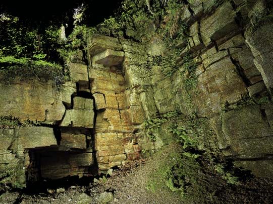
True color terrestrial laser scanning
A B
8.7m
C
E
1.750m
D
F
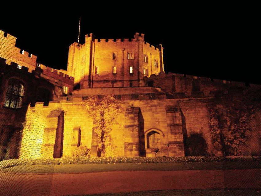
Figure 1. Terrestrial laser scan of an abandoned sandstone quarry in Carboniferous Coal Measures, County Durham.
(A) Scanning the outcrop with a Leica HDS 3000 scanner. (B) Resultant point cloud, showing gray scale points according
to intensity of the reflected beam. (C) Point cloud given false color according to the distance of each point from the scan
position. (D) Points in the point cloud allocated true color from tightly calibrated digital photos. (E) Close-up detail of
the gray scale point cloud. (F) Close-up of the colored point cloud, showing the extra stratigraphic detail now visible.
Vegetation is also more easily recognized in the colored point cloud.
Geosphere, June 2008 565
Downloaded from https://pubs.geoscienceworld.org/gsa/geosphere/article-pdf/4/3/564/3338879/i1553-040X-4-3-564.pdf
by guest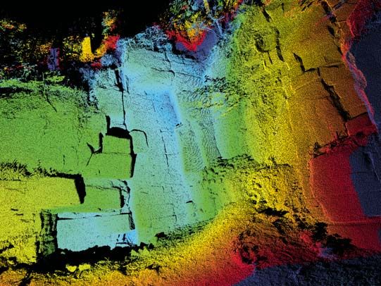
White and Jones

       as shown here is a colored point cloud, with brighter, more accurate color                      CAMERA MOUNT
       rendition compared with most existing TCTLS devices (which typically
       use a low-resolution onboard video camera to provide color data). This                             In order to minimize potential mismatch between the scan data and
       approach can also be extended to allow the mapped images to be draped                           color photos, a special camera mount was designed so that the optical
       onto a triangulated (meshed) surface derived from the point cloud (cf. Xu                       center of the camera can be positioned to align with the center of the laser
       et al., 2000; Bellian et al., 2005), so that the output is a textured model                     scanner. The essential feature of the mount is that it ensures that the center
       of the surface of the outcrop. This gives a model with even greater pixel                       of the entrance pupil of the camera lens remains coincident with the laser
       resolution and visible detail.                                                                  scanner center even when the camera is panned and tilted. A prototype
          While this work was particularly motivated by the aim to demonstrate                         mount was designed to be used with a Measurement Devices Ltd. (MDL)
       a prototype solution for a low-cost alternative to high-end commercial                          LaserAce 600 scanner. The mount accepts a wide range of cameras. The
       TCTLS, there were a number of additional reasons behind the project:                            camera can easily be adjusted on the mount within a range of positions,
          1. To be able to provide the best possible color-mapped point clouds                         although minor design modification to the dimensions of the mount was
       as input for new methods for automated feature recognition (e.g., auto-                         needed to make it suitable for use with some other makes of scanner. The
       mated removal of vegetation; extraction of fracture planes from the point                       mount was designed to fit the same standard tribrach fitting as the MDL
       cloud, c.f. Slob et al., 2005). Existing methods typically use only geomet-                     scanner and maintain the camera lens pivot point at the same height above
       rical analysis (e.g., edge and corner detection) and/or intensity contrasts.                    the tribrach as the scanner center. Thus the scanner can be removed from
       Supplementing feature recognition algorithms to exploit additional color                        the tripod once scanning is completed, and the camera mount attached in
       information has very interesting potential, but clearly relies on a precise                     its place, thereby ensuring that the laser scanner center and camera lens
       matching of the color data and point cloud as input.                                            pivot point are coincident.
          2. To provide a platform to allow a wider range of digital cameras to be                        To facilitate prototype design and fabrication, a rotating tribrach adapter
       used. For example, this has allowed us to test the use of lenses with longer                    (www.surveying.com/products/details.asp?prodID=2020-00) was used as
       focal lengths to capture very detailed photographs that can then be draped                      the base of the camera mount. As well as fitting the scanner tribrach, the
       onto meshed surfaces derived from the point cloud.                                              rotating tribrach adapter provided a flat surface with a good sized protrud-
          3. To allow for future development and testing of improved color map-                        ing thread in the center, and the rotation mechanism necessary for panning
       ping algorithms (e.g., to develop smoother color mapping in areas of over-                      the camera. The rest of the mount, fabricated from aluminum, was built on
       lapping images).                                                                                top of the adapter. A camera attaches to the mount using the standard ¼ in
          4. To be able to test the sensitivity of positioning of the camera with                      Whitworth (6.35 mm) thread tripod socket found on the base of most cam-
       respect to the laser scanner sensor. At present, some TCTLS devices (e.g.,                      eras. Figure 2 shows a rendered AutoCAD model of the as-built mount
       Riegl LMS scanners) use cameras mounted on top of the scanner body                              and a photograph of the mount with an SLR camera attached.
       (i.e., non-collinear with the laser scanner beam), and this introduces an                          The mount holds the camera in portrait format, partly because if a wide-
       error during matching of the photos with the point cloud data.                                  enough lens is used, a single photograph at each pan position will often
          5. To provide calibrated color outcrop models for benchmark compari-                         be sufficient, and partly because it would be difficult to design and manu-
       sons with other methods of building 3D outcrop models such as digital                           facture a mount that would hold the camera in landscape format and allow
       photogrammetry (e.g., Poropat, 2001; Pringle et al., 2001, 2004).                               the necessary panning and tilting while keeping the position of the center
          6. To have a precise, flexible system that is capable of mapping spa-                        of the entrance pupil constant. The design process was simplified by the
       tial data and imagery captured with alternative kinds of scanner and/                           fact that the majority of SLR cameras have their tripod sockets situated
       or camera device: e.g., for testing prototype scanners built with differ-                       directly below the longitudinal lens axis (when the camera is viewed in
       ent wavelengths or other laser properties, or for use with other types of                       landscape orientation). This meant that in the plate to which the camera is
       camera such as infrared or multi-spectral equipment (see also Bellian et                        attached, a simple slot with its centerline passing through the horizontal
       al., 2007).                                                                                     axis of rotation was sufficient to allow the center of the entrance pupil to
          7. To develop the necessary expertise to enable independent calibration                      be positioned in the horizontal rotational axis. Adjustments are therefore
       of camera lenses and testing of TCTLS performance.                                              only required in two axes in order to position the pivot point of the camera
          While a number of scanner manufacturers clearly have their own pro-                          lens in the vertical rotational axis.
       prietary methods to provide TCTLS, there is relatively little information                          The prototype camera mount described and used in this paper is non-
       available in the public domain that describes existing methods for color                        automated, such that the operator must manually reposition the camera
       mapping of laser scan data. Balis et al. (2004) implied how mapping                             around its rotation axes between each overlapping consecutive shot. Work
       is achieved using a Mensi GS200 scanner, which has internal onboard                             is under way to prototype a motorized version of the mount that will auto-
       video circuitry. Abmayr et al. (2004) used a specialized line-scanning                          matically take the photographs needed to cover a prescribed area.
       chromatic recorder to gather color information from the scanned area.
       Some workers have developed methods to combine scan data with pho-                              CAMERA CALIBRATION AND IMAGE RECTIFICATION
       tos taken with a standard digital single-lens reflex (SLR) camera from
       unspecified positions (i.e., scanner and camera need not be coincident                             Camera calibration and image rectification are well documented in rela-
       and collinear). Such methods typically minimize errors by using a large                         tion to applications in computer vision. Camera calibration is the process
       number of manually defined tie-points for each image (tie-points are                            of determining the internal camera geometric and optical characteristics
       points that can be located in both the rectified photographs and the                            (intrinsic parameters) and/or the 3D position and orientation of the camera
       point cloud). Examples of this approach include Xu et al. (2000), Gram-                         frame relative to a certain world coordinate system (extrinsic parameters)
       matikopoulos et al. (2004), and Abdelhafiz et al. (2005), although the                          (Tsai, 1987). It is not necessary to determine the extrinsic parameters in
       details of their methods are not all fully published. Abmayr et al. (2005)                      the TCTLS system described in this paper, because the camera is mounted
       give a comprehensive description of the use of such a method with the                           at the center of rotation of the laser scanner and tie-points are used to reg-
       Z+F 5003 scanner.                                                                               ister the images with the point cloud.

       566                                                                             Geosphere, June 2008

Downloaded from https://pubs.geoscienceworld.org/gsa/geosphere/article-pdf/4/3/564/3338879/i1553-040X-4-3-564.pdf
by guest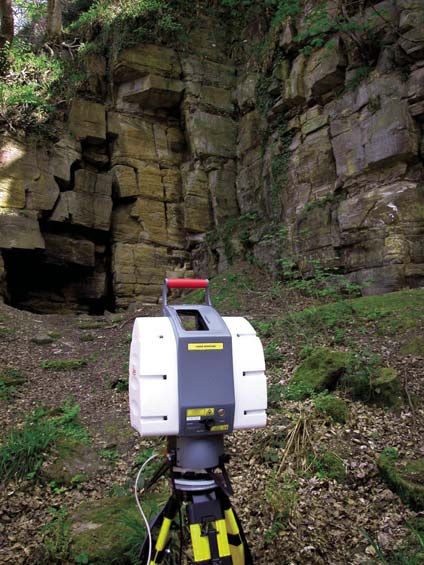
True color terrestrial laser scanning

                                 A                                                                         B

                              Figure 2. Rendered model of the as-built camera mount and a photograph of the mount with a single-lens reflex
                              camera attached. Height of mount is 36 cm.

                In order to register the photographs with the point cloud, the photo-
             graphs must be rectified such that they appear to have been captured with                                                                                                                              xis
                                                                                                                                                                                                               lA
             a pinhole camera, the pinhole of which is coincident with the laser-beam                                                                                  P                            ti    ca
                                                                                                                                                                                                 Op
             detector inside the laser scanner device. Figure 3 shows the pinhole cam-
                                                                                                                                           z
             era model with lens distortion, as well as how the laser scanner and image
             coordinate systems relate to each other. The orientation of the scanner                                                               y
             coordinate system about the vertical axis is arbitrary (for the MDL scan-
             ner used in this study it is defined by the direction in which the device is
             pointing when it is turned on).
                According to Heikkilä and Silvén (1997), the pinhole camera model is                                                                                              Ta
                                                                                                                                                                                     rg
                                                                                                                                                                                        e   tO
             based on the principle of collinearity, where each point in the object space                                                                                                     bje
                                                                                                                                                                       x                          c
             is projected by a straight line through the projection center into the image                                                                            Scanner                          t
                                                                                                                                                       Pl            Coordinate
             plane. Since after undistortion the photographs appear to have been cap-                                                     u            “Pane
                                                                                                                                                          inh o f    System
             tured with a pinhole camera, and if the camera-lens system is positioned                                           Q'                           ole
                                                                                                                                                                 ”
                                                                                                                                 Q
             such that the pinhole is coincident with the center of rotation of the laser                                             Pl
                                                                                                                     v                Caane
             scanner, then no further image rectification is required. Therefore it is nec-                              Im              me of
             essary to find the pinhole point for the camera-lens system. This point is                                  Coage              ra
                                                                                                                         Sy ord                Sen
                                                                                                                            ste ina                  so
             the center of perspective of the lens, about which the camera-lens sys-                                           m te                       r
             tem can be pivoted without introducing any parallax error between pho-
             tographs (Kerr, 2005). According to Kerr (2005), the correct pivot point
             is the center of the entrance pupil of the lens and not, contrary to popular                      Figure 3. Pinhole camera model with lens distortion, where P is a
             belief, the front nodal point. The center of the entrance pupil is easily                         three-dimensional subject point, Q is its distorted image point, and
             located empirically by observing the relative movement of the background                          Q' is its undistorted image point (Shih et al., 1995).

                                                                                             Geosphere, June 2008                                                                                              567

Downloaded from https://pubs.geoscienceworld.org/gsa/geosphere/article-pdf/4/3/564/3338879/i1553-040X-4-3-564.pdf
by guest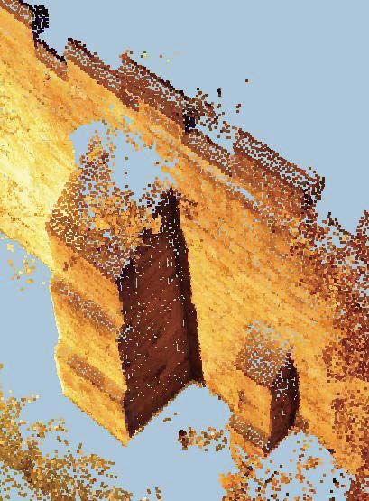
White and Jones

       and foreground as the camera is pivoted about different points. The point                       rotates about the vertical axis and is, therefore, the angle between the azi-
       at which there is no relative movement between the background and fore-                         muth zero line in the horizontal plane and the projection of the subject
       ground is the correct pivot point.                                                              point onto the same plane. This is not the same as the horizontal angle
          The intrinsic parameters required to rectify the image to achieve this                       between the subject point and the vertical plane that passes through the
       pinhole camera model are usually the effective focal length, scale factor,                      azimuth zero line. The inclination is simply the direct angle between the
       and image center (principal point), as well as those needed to correct for                      horizontal plane passing through the image center and the subject point.
       the systematically distorted image coordinates (Heikkilä and Silvén, 1997).                        The implications of the method of operation of the laser scanner can
       The main type of distortion is radial distortion, in which the actual image                     be understood by considering the lines traced out by the laser beam on
       point is shifted radially in the image plane. In addition, a decentring distor-                 the inside of a virtual sphere when θ or φ is kept constant, given that the
       tion with both radial and tangential components occurs due to the centers of                    laser scanner center is at the center of the sphere. If the inclination is kept
       curvature of lens surfaces not being collinear. Figure 4 illustrates the effects                constant while the azimuth is varied, a line of “latitude” is traced on the
       of radial and decentring distortions on a synthetic image.                                      surface of the sphere. If, instead, the azimuth is kept constant while the
          A number of methods have been documented for determining the dis-                            inclination is varied, a line of “longitude” is traced on the surface.
       tortion parameters empirically. One example of an application for cam-                             The interaction of the laser scanner and the camera can be understood
       era calibration and image rectification is the GML (Graphics and Media                          by imagining the projections of the lines of latitude and longitude onto a
       Lab) C++ Camera Calibration Toolbox (v. 0.31 or later) by Vezhnevets                            virtual plane external to the sphere by straight lines passing through the
       and Velizhev (2005, 2006). This application has been tested with the                            center of the sphere. If the plane is vertical, the lines of latitude above the
       TCTLS solution presented in this paper, although any alternative method                         equator map to upward-curving lines on the plane, and those below the
       that adequately removes distortion from the photographs can be used as                          equator map to downward-curving lines. The lines of longitude, however,
       part of the system. Vezhnevets and Velizhev’s (2005, 2006) toolbox is an                        map to vertical lines on the plane. If the plane is now tilted upward, the
       implementation in C++ of a Matlab toolbox by J.-Y. Bouguet (www.vision.                         projected lines of latitude now all curve upward, as long as the bottom
       caltech.edu/bouguetj/calib_doc/download/TOOLBOX_calib.zip), with the                            of the virtual plane is above the equatorial plane. The projections of the
       addition of another corner detection algorithm. Both toolboxes use an                           lines of longitude remain straight, but splay out toward the bottom of the
       intrinsic camera model inspired by Heikkilä and Silvén (1997), and a main                       plane. If the plane is tilted downward, the projected lines of latitude curve
       initialization phase partially inspired by Zhang (2000) and partially devel-                    downward and the projections of the lines of latitude splay out toward the
       oped by Bouguet (both available from the Intel Open Source Computer                             top of the plane. This is illustrated in Figure 6.
       Vision Library at www.intel.com/technology/computing/opencv). Unlike                               Since the scanner is an inherently spherical system using polar coor-
       Bouguet’s toolbox, Vezhnevets and Velizhev’s (2005, 2006) software is                           dinates, and the camera sensor is a plane, the scanner-camera system
       capable of rapidly undistorting large, high-resolution images.                                  conforms to this behavior, with the virtual image plane corresponding to
          In order to calibrate a camera, a set of photographs is taken of a planar                    the camera’s sensor. When the virtual plane in Figure 6 is vertical, this
       “checkerboard” calibration target. The toolbox is able to detect the corners                    corresponds to the case in which the camera’s sensor is vertical, i.e., the
       of the squares in the photographs of the target and use their positions to                      longitudinal axis of the lens is pointing horizontally. Similarly, when the
       calculate the intrinsic calibration parameters. Any photographs taken with                      virtual plane is inclined, this corresponds to the situation in which the
       the same camera and lens (at the same focal length, if it is a zoom lens)                       camera is tilted about a horizontal line passing through the laser-beam
       can then be undistorted using the toolbox, whether or not the photographs                       detector (i.e., center of the scanner) and the camera lens pivot point. From
       were taken before the calibration was carried out.                                              Figure 6 it can be deduced that in the case where the lens is pointing hori-
                                                                                                       zontally, the expression for v will be a function of both θ and φ, while u
       COREGISTRATION OF COLOR IMAGES AND SCAN DATA                                                    will be a function of θ only. In the tilted case, however, both u and v are
                                                                                                       functions of both θ and φ. This information is summarized in Table 1. A
          In order to register an image with a point cloud, a mapping must be
       determined that gives expressions for the image pixel coordinates u and
       v (Fig. 5), in terms of the azimuth (horizontal) and inclination (vertical)                                                         u
       angles, θ and φ, respectively, from the laser scanner center to the corre-
       sponding point in the cloud.
          It is important to note the way in which laser scanners measure the
       azimuth and inclination angles. The azimuth is measured as the scanner
                                                                                                                            v
                                                                                                                                                              V

                                                                                                                                           U
                                                                                                                     Figure 5. Coordinate system of the rec-
                Original                     Radial Distortion               Decentring Distortion                   tified image plane. U and V are the total
                                                                                                                     number of horizontal and vertical pixels
                                                                                                                     in the image, respectively; u and v are the
       Figure 4. Effects of radial and decentring distortions on a synthetic                                         pixel coordinates relative to the top left
       image (Prescott and McLean, 1997).                                                                            corner of image.

       568                                                                             Geosphere, June 2008

Downloaded from https://pubs.geoscienceworld.org/gsa/geosphere/article-pdf/4/3/564/3338879/i1553-040X-4-3-564.pdf
by guest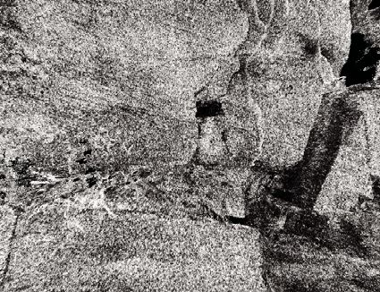
True color terrestrial laser scanning
5. Mapping color values from the images onto the point cloud. This is
done by using Newton’s method to solve the three simultaneous nonlinear
equations as derived in the Appendix.
6. Saving an output file of point cloud data, now comprising x, y, and z
ф = constant ф = constant
θ = constant θ = constant ф = constant coordinates and RGB (red green blue) color values.
θ = constant The point cloud data can thus be suitably colored and can be imported
into appropriate visualization software, such as the open-source program
ParaView (www.paraview.org).
TESTING THE SYSTEM
To test the system a number of field tests were performed, using a vari-
ety of laser scanners and cameras. In the first tests, buildings were mainly
Plane Vertical Plane Inclined Upwards Plane Inclined Downwards
used as the chosen target objects, because they have distinct geometric
features that can readily be checked in both the scan data and photographs.
Figure 6. Projections of lines of constant azimuth and inclination Later tests used geological outcrops.
onto vertical and inclined planes. In the first field test illustrated here, part of Durham Castle was chosen
to provide a target with complicated geometry. For this test the laser scan-
ner chosen was a Riegl LMS-Z420i, which has its own in-built function
TABLE 1. FORM OF MAPPING FUNCTIONS for high-quality color matching through the use of a separate precision-
mounted digital SLR on top of the scanner. A 360° scan was acquired,
Camera horizontal Camera tilted consisting of 8 × 10⁶ points. Two separate sets of photographs were
u = f (θ) u = f ( θ, ф ) acquired, to allow direct comparison between our method of color match-
v = f ( θ, ф) v = f (θ ,ф) ing and that provided by Riegl. The first set of 7 photographs was taken
Note: u—horizontal image pixel coordinate; with a top-mounted 6.1 mega-pixel Nikon D70 camera (giving a total of
v—vertical image pixel coordinate; θ—azimuth 42.7 × 106 pixels), following Riegl’s standard acquisition method for the
(horizontal) angle; ф—inclination (vertical) scanner. The scanner was then removed from the tripod, and a second set
angle. of 18 photos was taken using an 8 mega-pixel Canon EOS 350D together
with the camera mount and color matching method presented in this paper
(total pixels = 144 × 106). Figure 7 shows the quality of the colored point
cloud matching for part of the castle. Color matching is very precise in all
full mathematical derivation of the actual mapping functions is given in areas of the photos, including objects in the near foreground and far back-
the Appendix. ground (this is difficult to achieve when the camera is not collinear with
the scanner center, as in the top-mounted Riegl scanners). This benchmark
COREGISTRATION TOOLBOX test shows that the color matching method we present in this paper can
perform at least as well as high-end commercial solutions.
The Matlab programming environment was used to create a set of The second example shown here is from the Jurassic coastal cliff sec-
tools that can be used to carry out the registration process of a set of tions at Staithes, North Yorkshire. This site is part of a long-term project
photographs with its associated point cloud. The toolbox comprises a using laser scanning to monitor coastal erosion (Rosser et al., 2005; Lim
number of individual programs collectively controlled through a com- et al., 2005). In this test an MDL LaserAce 600 scanner and an Olympus
mon Graphical User Interface (GUI). The toolbox encompasses the fol- Camedia E-20P digital SLR camera were used. The results (Fig. 8) show
lowing functionality. that color matching has high precision, and that the addition of color to the
1. Loading and parsing of the raw ASCII laser scan point cloud file point cloud greatly increases the amount of geological detail visible in the
(comprising the x, y, and z Cartesian coordinates for each point). virtual outcrop model.
2. Conversion of the points from Cartesian coordinates to a spherical
reference frame with the center of the scanner (and camera) at the origin. ERROR ANALYSIS
The azimuth and inclination coordinates are calculated from the x, y, and
z coordinates using the following formulae: There are many stages in the data capture and image registration pro-
cesses, some of which introduce errors. Quantitative aspects of the fol-
lowing error analysis are specific to the MDL LaserAce 600 scanner and
⎛ x⎞
azimuth = arctan ⎜ ⎟ Olympus Camedia E-20P camera, but other scanner and camera combina-
⎝ y⎠ (1) tions are conceptually similar.
A significant source of error can arise because of dispersion of the scan-
and ner’s laser beam. The scanner assumes that the strongest part of the return-
⎛ z ⎞ ing beam originates from the center of the laser-beam footprint on the
inclination = arctan ⎜ 2 ⎟ . (2) target, but when the footprint overlaps areas of contrasting reflectance,
⎝ x +y ⎠
2
this concentric weighting is distorted. The effects of this error are usually
most noticeable at the edges of objects that have sky (or distant back-
3. Loading of the corrected (i.e., undistorted) images. ground beyond the range of the scanner) behind them, and is often seen as
4. Input of the tie-point coordinates. a band of sky-colored points (typically one point wide) extending around
Geosphere, June 2008 569
Downloaded from https://pubs.geoscienceworld.org/gsa/geosphere/article-pdf/4/3/564/3338879/i1553-040X-4-3-564.pdf
by guest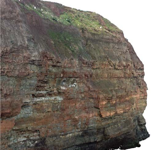
White and Jones

         A                                                                                           B                                                 C

                                                                                                                                                       D

       Figure 7. Colored point cloud of part of Durham Castle. (A) Screenshot of three-dimensional model visualized using ParaView software. (B)
       Oblique view with areas of scan shadow. (C, D) Areas of detail where crenellations, buttresses, and windows reveal the quality of the color map-
       ping. Vertical distance from courtyard to top of flag post is 49.4 m. Width of window lintel in (C) is 2.22 m. Height of wall in (D) is 6.05 m.

       the edge of the scanned object. When a dispersed beam hits the edge of an                          Other sources of error relate to the discrepancy between the color of
       object, part of the beam footprint is reflected and recorded by the scanner,                    the point in the point cloud and the color of the corresponding point in the
       even though the center of the beam footprint was in the sky. The scanner                        subject, i.e., errors in the registration of the images with the point cloud.
       therefore captures a data point beyond the edge of the object, even though                      In order to quantify the maximum registration error, approximate expres-
       that point does not actually exist. When the resolution of the accompany-                       sions were derived for the angular errors at different stages in the capture
       ing photo is high relative to the spacing of points in the point cloud, a thin                  and registration of the color information.
       band of sky is mapped onto the extra trace of spurious points that flank                           The maximum angular registration error, αreg, is given by:
       the true edge of the object. This source of error is common to all scanners
       that have wide beam dispersion. It needs to be taken into consideration                                      α reg = α pos + α rot + α rect + α tie ,             (3)
       because the error is caused by an intrinsic property of the scanner, and is
       not related to poor camera calibration or image matching.                                       where αpos is the angular error due to positioning the center of the entrance
          A second source of error can arise due to occlusion. Lim et al. (2005)                       pupil of the lens coincident with the beam detector of the laser scanner;
       carried out an experiment using the same MDL LaserAce 600 scanner                               αrot is due to the deviation from vertical of the plate to which the camera
       used to capture the point clouds in Figure 8. They scanned a section of                         attaches on the mount; αrect is the error in the rectification process using
       cliff at 0.05° resolution twice in immediate succession and quantified the                      the GML toolbox; and αtie is due to the human judgment error in locating
       discrepancies between the two scans due to occlusion errors. Occlusion                          the tie-points in the gray scale or false color point cloud. αpos and αrect were
       errors are due to problems resulting from scanning a complex surface,                           quantified by making assumptions about the magnitude of tolerances and
       in which some surface data are missed and, therefore, interpolated. The                         analytically deriving expressions for the resulting errors. αrot was deter-
       errors, which are concentrated toward the edges of the scans and on pro-                        mined by empirically measuring the effect of an artificially applied rota-
       truding ledges, occur due to the occluded data being interpolated differ-                       tion and αtie was based on empirical observation.
       ently during successive scans. Despite these errors, Lim et al. (2005) stated                      When the expressions for these individual errors are substituted into the
       that point cloud data acquired with the MDL LaserAce 600, over ranges                           above equation, the following expression is obtained for αreg, in degrees:
       typically associated with scanning cliff faces, are capable of accuracies
       within ±0.06 m. This error is the maximum error between the position of
                                                                                                                      ⎛ 0.0025 ⎞
       a subject point in space and the coordinates of the corresponding point in                      α reg ≈ arctan ⎜          + 0.45β + 0.017 + ( 0.5 − 0.45G ) ,
                                                                                                                      ⎝ D ⎟⎠
                                                                                                                                                                         (4)
       the point cloud. The magnitude of this error is purely related to the scan-
       ner; a higher quality scanner would give greater accuracy.

       570                                                                             Geosphere, June 2008

Downloaded from https://pubs.geoscienceworld.org/gsa/geosphere/article-pdf/4/3/564/3338879/i1553-040X-4-3-564.pdf
by guest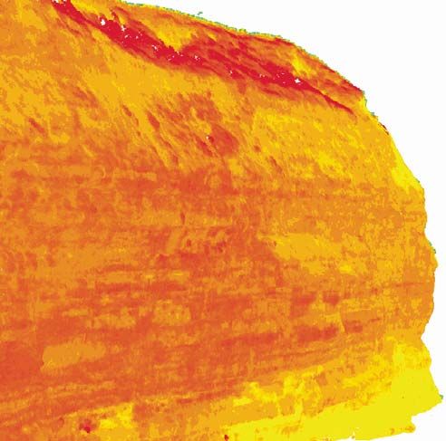
True color terrestrial laser scanning

                          A                                                                                    B

                          C                                                                                    D

                       Figure 8. Laser scan point cloud data from a project to monitor coastal erosion at Staithes, North Yorkshire (Rosser et al.,
                       2005). (A) Scanning the outcrop with an MDL LaserAce 600 scanner. (B) Gray scale point cloud based on the intensity of the
                       reflected laser beam. (C) False color red-yellow ramp applied to intensity values (replacing the gray scale) for each point. (D)
                       True color point cloud significantly helps to emphasize the geological detail in the outcrop. Height of cliff is 35.5 m.

             where D is the distance to the subject in meters; β is the rotation of the                       αreg is conservative. With G equal to unity, by far the most significant term
             camera from vertical in degrees; and G is a subjective “geometricity”                            in the above expression is αrot, contributing 57% of the maximum regis-
             coefficient. For a subject with distinct geometric features, such as a simple                    tration error of 0.16° when β = 0.2° and D = 5 m, and 72% of the 0.25°
             building, G would take the value 1, whereas for a very irregular subject,                        maximum registration error when β = 0.4° and D = 70 m. To combat this
             such as a cliff face, G would take a value of 0. If necessary, however, αtie                     error, the camera mount design could be modified so that it is stiffened, in
             can be virtually eliminated by adjusting the image registration by altering                      order to reduce the distortion due to the weight of the camera. Better still
             the three mapping parameters. To obtain the approximate maximum regis-                           would be the addition of a mechanism for providing a fine adjustment to
             tration error in terms of a number of points, αreg should be divided by the                      ensure that the camera is truly vertical. This would greatly reduce the rota-
             resolution of the scanner in degrees.                                                            tion error, and therefore the registration error.
                Although it was necessary to make some fairly crude assumptions in                               The above expression was derived to give an approximate maxi-
             order to derive some of the individual errors, the resulting expression for                      mum limit on the registration error. In practice, the errors observed are

                                                                                             Geosphere, June 2008                                                                     571

Downloaded from https://pubs.geoscienceworld.org/gsa/geosphere/article-pdf/4/3/564/3338879/i1553-040X-4-3-564.pdf
by guest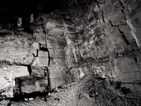
White and Jones

       significantly less than αreg over most of the point cloud. Over those areas                        The level of accuracy with which the photographs can be registered with
       of the point cloud colored by pixels from near edges of the photographs,                        the point cloud is such that the resulting true color point cloud can support
       the errors approach αreg. This error analysis will allow comparisons to be                      very detailed analysis and data interpretation for many applications. The
       drawn with associated technologies, such as photogrammetry, as well as                          ability to adjust the registration of the photographs with the point cloud
       helping to prevent inappropriate use of the data.                                               has considerable benefits when scanning irregular subjects such as cliff
                                                                                                       faces, which generally have few geometrically regular features.
       CONCLUSIONS                                                                                        Detailed error analysis enables comparisons to be drawn with related
                                                                                                       technologies, as well as with commercially available true color terrestrial
          A low-cost true color terrestrial laser scanning (TCTLS) system has                          laser scanners. The accuracy of the registration is comparable with that of
       been developed for use in a wide variety of applications. The low cost of                       commercially available TCTLS devices. This novel, low-cost, accurate,
       this system makes TCTLS technology more financially viable to a larger                          and flexible TCTLS technology has the potential to make a significant
       number of people in a greater range of fields. The flexibility of the system                    impact on the spatial data acquisition capabilities of many companies and
       also provides a useful platform for further research into TCTLS to test per-                    academic institutions. We hope that this paper will provide the basis for
       formance of a range of digital cameras, lenses, and laser scanner devices.                      further research and development in the fields of low-cost TCTLS and the
          True color capability can be added to existing terrestrial laser scanners                    analytic mapping approach, and that it has the potential to lead to the com-
       using a purpose-built camera mount and coregistration software. The camera                      mercial implementation of a user-friendly, low-cost, true color terrestrial
       mount allows the photographs to be captured from exactly the same point as                      laser scanning system.
       the point cloud and, in doing so, reduces one source of error present in some
       commercial laser scanners that use top-mounted cameras. Using a digital                         APPENDIX
       SLR, rather than onboard video circuitry mounted inside the scanner, pro-
       vides higher resolution images, and gives more faithful chromatic data.                            First, the mapping functions for the horizontal case will be derived. These func-
          The use of an adjustable camera mount, which takes a range of cam-                           tions are then extended to account for the case where the camera is tilted. Finally, a
                                                                                                       method is determined for solving the resulting functions for a pair of tie-points for
       eras, allows the user flexibility over the hardware used to capture the data.                   each image. Figure 9 shows the relationship between the laser scanner coordinate
       Further work is under way to construct an automated system prototype                            system and the virtual image plane with its coordinate system. The laser scanner
       that applies the same principles of image and/or scan coregistration to a                       center and the virtual image plane are separated by a virtual distance, d, perpen-
       motorized version of the camera mount.                                                          dicular to the plane. θc is the angle from the azimuth zero line to the center of the
                                                                                                       virtual image plane, and u' and v' define an alternative image coordinate system
          The calibration of the camera is simple and quick, using a stiff planar                      with respect to an origin at the center of the virtual image plane.
       checkered calibration target and standard camera calibration algorithms.                        Deriving an expression for u in the horizontal case, considering triangle OAC:
       There is no requirement for the camera to be calibrated prior to taking the
       photographs, and each camera and lens need only be calibrated once. The
                                                                                                                                          u′
       undistortion process is fast and allows a batch of images to be undistorted                                     tan ( θ − θc ) =        .                              (5)
       with one click of a mouse.                                                                                                         d

                           Figure 9. Relationship between the laser scanner and the virtual image plane in the case where the lens is
                           pointing horizontally. See text for definition of symbols.

       572                                                                             Geosphere, June 2008

Downloaded from https://pubs.geoscienceworld.org/gsa/geosphere/article-pdf/4/3/564/3338879/i1553-040X-4-3-564.pdf
by guest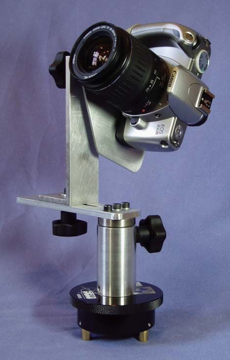
True color terrestrial laser scanning

             Converting between u' and u:                                                                     In order to derive expressions for u and v in the case where the camera is tilted at
                                                                                                              an angle θc to the horizontal, the coordinate system shall be rotated by θc about the
                                                                                                              y axis. The rotation matrix required to perform the rotation by angle φc about the
                                                U
                                    u′ = u −      .                                       (6)                 y axis is:
                                                2
                                                                                                                            ⎡ cos φ c      0 sin φ c ⎤
                                                                                                                            ⎢ 0
             Substituting for u' in equation 5:
                                                                                                                            ⎢              1   0 ⎥⎥ .                                (16)
                                                u −U                                                                        ⎢⎣ − sin φ c   0 cos φ c ⎥⎦
                             tan ( θ − θc ) =          2 .                                (7)
                                                   d

             Rearranging:

                                  U
                             u=     + d tan ( θ − θc ) .                                  (8)
                                  2

             Deriving an expression for v in the horizontal case, considering the triangle defined
             by O, A, and the point (u, v):

                                                v′
                                    tan φ =        .                                      (9)
                                                l

             Considering triangle OAC:

                                                   d
                                cos ( θ − θc ) =     .                                    (10)
                                                   l

             Rearranging:

                                l = d sec ( θ − θc ) .                                    (11)

             Converting between v' and v:
                                                                                                              Figure 10. Relationship between the laser scanner and virtual image
                                        V                                                                     plane in the general case where the camera is tilted. See text for
                                    v′ = − v .                                            (12)
                                        2                                                                     definition of symbols.

             Substituting for v' and l in equation 9:
                                                                                                                                                          z
                                          V −v
                             tan φ =        2
                                                        .                                 (13)
                                       d sec ( θ − θc )
                                                                                                                                                                     (x,y,z)
             Rearranging:
                                                                                                                                                                               y
                               V
                          v=     − d sec ( θ − θc ) tan φ .                               (14)                                                                   ф
                               2
                                                                                                                                                  θc
                                                                                                                                                                  θ
             Next, the general case in which the camera can be tilted at an angle to the horizontal                                                               x
             is considered. Figure 10 shows the relationship between the laser scanner coordi-
             nate system and the image plane coordinate system in the tilted case.
                First, converting between Cartesian coordinates and spherical polar coordinates
             as defined in Figure 11:

                           ⎡ x ⎤ ⎡ cos ( θ − θc ) cos φ ⎤
                           ⎢ y ⎥ = ⎢ sin θ − θ cos φ ⎥ .
                           ⎢ ⎥ ⎢ (             c)
                                                                                          (15)                Figure 11. Relationship between Cartesian coordinate system and
                                                        ⎥
                           ⎢⎣ z ⎥⎦ ⎢⎣                   ⎥                                                     spherical polar coordinate system on a sphere of unit radius. See
                                           sin φ        ⎦                                                     text for definition of symbols.

                                                                                             Geosphere, June 2008                                                                             573

Downloaded from https://pubs.geoscienceworld.org/gsa/geosphere/article-pdf/4/3/564/3338879/i1553-040X-4-3-564.pdf
by guest
White and Jones
Therefore, premultiplying the matrix on the right side of equation 15 by the rotation
matrix above:
v=
V d ( sec ( θ − θc ) tan φ − tan φ c
−
) . (25)
2 1 + sec ( θ − θc ) tan φ tan φ c
⎡ cos ( θ′ − θc ) cos φ ′ ⎤ ⎡ cos φ c 0 sin φ c ⎤ ⎡ cos ( θ − θc ) cos φ ⎤
⎢ ⎥ ⎢ ⎢ ⎥
⎢ sin ( θ′ − θc ) cos φ ′ ⎥ = ⎢ 0 1 0 ⎥⎥ ⎢ sin ( θ − θc ) cos φ ⎥ Now a method of solution of equations 24 and 25 is described that can be imple-
mented algorithmically (e.g., in a Matlab program).
⎢ ⎥ 0 cos φ c ⎥⎦ ⎢⎣ ⎥
⎣ sin φ ′ ⎦ ⎢⎣ − sin φ c sin φ ⎦ For each image, if the u, v coordinates of two points in the image and the corre-
sponding θ, φ coordinates of the same two points in the point cloud are known, and
given the horizontal and vertical pixel dimensions of the image, then four equations
⎡ cos ( θ′ − θc ) cos φ ′ ⎤ ⎡ cos φ c cos ( θ − θ c ) cos φ + sin φ c sin φ ⎤ can be formed containing only three unknown mapping parameters, θc, φc, and d:
⎢ ⎥ ⎢ ⎥ . (17)
⎢ sin ( θ′ − θc ) cos φ ′ ⎥ = ⎢ sin ( θ − θc ) cos φ Tie-points (u1, v1, θ1, φ1) and (u2, v2, θ2, φ2):
⎥
⎢ sin φ ′ ⎥ ⎢ cos φ c sin φ − sin φ c cos ( θ − θc ) cos φ ⎥
⎣ ⎦ ⎣ ⎦
U d tan ( θ1 − θc ) sec φ c
u1 = + (26)
The equations corresponding to equations 8 and 14 for the tilted case are: 2 1 + sec ( θ1 − θc ) tan φ1 tan φ c
U
u= + d tan ( θ′ − θc )
2
(18) U d tan ( θ2 − θc ) sec φ c
u2 = + (27)
and 2 1 + sec ( θ2 − θc ) tan φ 2 tan φ c
V
− d sec ( θ′ − θc ) tan φ ′ . )
V d ( sec ( θ1 − θc ) tan φ1 − tan φ c
v= (19)
2 v1 = − (28)
2 1 + sec ( θ1 − θc ) tan φ1 tan φ c
Using equation 17 to express tan(θ'– θc) in terms of θ, φ, θc, and φc:
v2 =
V d ( sec ( θ2 − θc ) tan φ 2 − tan φ c
−
)
sin ( θ′ − θc ) cos φ ′ 1 + sec ( θ2 − θc ) tan φ 2 tan φ c
. (29)
tan ( θ′ − θc ) = 2
cos ( θ′ − θc ) cos φ ′
Only three of these equations are required in order to solve for the three mapping
parameters.
sin ( θ − θc ) cos φ If the three simultaneous nonlinear equations 26, 27, and 28 are rearranged
= . (20)
cos φ c cos ( θ − θc ) cos φ + sin φ c sin φ thus:
U d tan ( θ1 − θc ) sec φ c
Similarly, using equation 17 to express sec(θ'– θc) tan φ in terms of θ, φ, θc, and φc: f ( θc , φ c , d ) = − u1 + (30)
2 1 + sec ( θ1 − θc ) tan φ1 tan φ c
sin φ ′
sec ( θ′ − θc ) tan φ ′ =
cos ( θ′ − θc ) cos φ ′ U d tan ( θ2 − θc ) sec φ c
g ( θc , φ c , d ) = − u2 + (31)
2 1 + sec ( θ2 − θc ) tan φ 2 tan φ c
cos φ c sin φ − sin φ c cos ( θ − θc ) cos φ
=
cos φ c cos ( θ − θc ) cos φ + sin φ c sin φ
. (21)
h ( θc , φ c , d ) =
V
− v1 −
d ( sec ( θ1 − θc ) tan φ1 − tan φ c ) , (32)
2 1 + sec ( θ1 − θc ) tan φ1 tan φ c
Multiplying numerator and denominator of both the above expressions by sec φc
sec(θ – θc) sec φ: then they can be solved by using Newton’s method (http://numbers.computation
.free.fr/Constants/Algorithms/newton.html) in the following form:
tan ( θ − θc ) sec φ c
tan ( θ′ − θc ) = (22) ⎡ θc ⎤ ⎡ θc ⎤ ⎡ f ( θc , φ c , d ) ⎤
1 + sec ( θ − θc ) tan φ tan φ c
⎢ φ ⎥ = ⎢ φ ⎥ − J −1 θ , φ , d ⎢ g θ , φ , d ⎥ ,
⎢ c⎥ ⎢ c⎥ ( c c ) ⎢ ( c c )⎥ (33)
⎢⎣ d ⎥⎦ n +1 ⎢⎣ d ⎥⎦ n ⎢ h ( θc , φ c , d ) ⎥
sec ( θ − θc ) tan φ − tan φ c ⎣ ⎦n
sec ( θ′ − θc ) tan φ ′ = . (23)
1 + sec ( θ − θc ) tan φ tan φ c where J is the Jacobian matrix:
⎡ ∂f ∂f ∂f ⎤
Substituting for tan(θ´– θc) from equation 22 into equation 18, and for sec(θ′ – θc) ⎢ ⎥
tan φ′ from equation 23 into equation 19 to give expressions for u and v for the ⎢ ∂θc ∂φ c ∂d ⎥
tilted case: ⎢ ∂g ∂g ∂g ⎥
J ( θc , φ c , d ) = ⎢ ⎥
U d tan ( θ − θc ) sec φ c ⎢ ∂θc ∂φ c ∂d ⎥ . (34)
u= + (24) ⎢ ∂h ∂h ∂h ⎥
2 1 + sec ( θ − θc ) tan φ tan φ c ⎢ ⎥
⎣ ∂θc ∂φ c ∂d ⎦
574 Geosphere, June 2008
Downloaded from https://pubs.geoscienceworld.org/gsa/geosphere/article-pdf/4/3/564/3338879/i1553-040X-4-3-564.pdf
by guestTrue color terrestrial laser scanning
ACKNOWLEDGMENTS Labourdette, R., and Jones, R.R., 2007, Characterization of fluvial architectural elements
using a three dimensional outcrop dataset: Escanilla braided system—South-central
Pyrenees, Spain: Geosphere, v. 3, p. 422–434, doi: 10.1130/GES00087.1.
We thank John Parker for his help with the analytical mapping, and Nick Rosser,
Lim, M., Petley, D.N., Rosser, N.J., Allison, R.J., Long, A.J., and Pybus, D., 2005, Com-
Alan Purvis, David Toll, Roger Little, Nick Holliman, and Steve Waggott (Hal- bined digital photogrammetry and time-of-flight laser scanning for monitoring cliff
crow) for their help and insight. We also thank Jerry Bellian and Klaus Gessner for evolution: Photogrammetric Record, v. 20, no. 110, p. 109–129, doi: 10.1111/j.1477-
useful reviews, as well as Tim Wawrzyniec and Randy Keller for editorial input. 9730.2005.00315.x.
Aspects of material presented in this paper are protected under UK and Interna- Løseth, T.M., Thurmond, J., Søegaard, K., Rivenæs, J.C., and Martinsen, O.J., 2003, Build-
tional Patent laws. ing reservoir model using virtual outcrops: A fully quantitative approach: American
Association of Petroleum Geologists, International Meeting, Programs with Abstracts,
Salt Lake City, Utah, May 9–14.
REFERENCES CITED
McCaffrey, K.J.W., Jones, R.R., Holdsworth, R.E., Wilson, R.W., Clegg, P., Imber, J., Hol-
liman, N., and Trinks, I., 2005, Unlocking the spatial dimension: Digital technologies
Abdelhafiz, A., Riedel, B., and Niemeier, W., 2005, Towards a 3D true coloured space by the and the future of geoscience fieldwork: Geological Society [London] Journal, v. 162,
fusion of laser scanner point cloud and digital photos, in El-Hakim, S., et al., eds., Vir- p. 927–938, doi: 10.1144/0016-764905-017.
tual reconstruction and visualization of complex architectures: International Archives of Prescott, B., and McLean, G.F., 1997, Line-based correction of radial lens distortion: Graphical
Photogrammetry, Remote Sensing, and Spatial Information Sciences, v. 36, part 5/W17, Models and Image Processing, v. 59, no. 1, p. 39–47, doi: 10.1006/gmip.1996.0407.
http://www.commission5.isprs.org/3darch05/pdf/31.pdf (August 30, 2007). Poropat, G.V., 2001, New methods for mapping the structure of rock masses, in Proceedings,
Abmayr, T., Härtl, F., Mettenleiter, M., Heinz, I., Hildebrand, A., Neumann, B., and Fröhlich, Australian Institute of Mining and Metallurgy Conference, EXPLO2001, Hunter Valley,
C., 2004, Realistic 3D reconstruction—Combining laserscan data with RGB color NSW, Australia.
information: International Archives of Photogrammetry, Remote Sensing, and Spa- Pringle, J.K., Clark, J.D., Westerman, A.R., Stanbrook, D.A., Gardiner, A.R., and Morgan,
tial Information Sciences, v. 35, part B5, http://www.isprs.org/istanbul2004/comm5/ B.E.F., 2001, Virtual outcrops: 3-D reservoir analogues, in Ailleres, L., and Rawling, T.,
papers/549.pdf (August 30, 2007). eds., Animations in geology: Journal of the Virtual Explorer, v. 3, http://virtualexplorer
Abmayr, T., Dalton, G., Hines, D., Liu, R., Härtl, F., Hirzinger, G., and Fröhlich, C., 2005, .com.au/journal/2001/04/pringle/
Standardization and visualization of 2.5D scanning data and color information by Pringle, J.K., Westerman, A.R., Clark, J.D., Drinkwater, N.J., and Gardiner, A.R., 2004, 3D
inverse mapping, in Proceedings, Conference on Optical 3D Measurement Techniques, high-resolution digital models of outcrop analogue study sites to constrain reservoir
7th, Vienna, Austria: TU Wien, p. 164–173. model uncertainty: An example from Alport Castles, Derbyshire, UK: Petroleum Geo-
Ahlgren, S., and Holmlund, J., 2002, Outcrop scans give new view: American Association of science, v. 10, p. 343–352.
Petroleum Geologists Explorer, p. 22–23. Pringle, J.K., Hodgetts, D., Howell, J.A., and Westerman, A.R., 2006, Virtual outcrop models
Balis, V., Karamitsos, S., Kotsis, I., Liapakis, C., and Simpas, N., 2004, 3D-laser scanning: Inte- of petroleum reservoir analogues—A review of the current state-of-the-art: First Break,
gration of point cloud and CCD camera video data for the production of high resolution v. 24, p. 33–42.
and precision RGB textured models: Archaeological monuments surveying application Rosser, N.J., Petley, D.N., Lim, M., Dunning, S.A., and Allison, R.J., 2005, Terrestrial
in ancient Ilida, in Proceedings, FIG Working Week, Athens, Greece, May 22–27, 2004: laser scanning for monitoring the process of hard rock coastal cliff erosion: Engi-
http://www.fig.net/pub/athens/papers/wsa2/WSA2_5_Balis_et_al.pdf (August 30, 2007). neering Geology and Hydrogeology Quarterly Journal, v. 38, p. 363–375, doi:
Barber, D.M., Dallas, R.W.A., and Mills, J.P., 2006, Laser scanning for architectural conser- 10.1144/1470-9236/05-008.
vation: Journal of Architectural Conservation, v. 12, p. 35–52. Shih, S.W., Hung, Y.P., and Lin, W.S., 1995, When should we consider lens distor-
Bellian, J.A., Kerans, C., and Jennette, D.C., 2005, Digital outcrop models: Applications of tion in camera calibration: Pattern Recognition, v. 28, no. 3, p. 447–461, doi:
terrestrial scanning lidar technology in stratigraphic modelling: Journal of Sedimentary 10.1016/0031-3203(94)00107-W.
Research, v. 75, p. 166–176, doi: 10.2110/jsr.2005.013. Slob, S., and Hack, R., 2004, 3D terrestrial laser scanning as a new field measurement and
Bellian, J.A., Beck, R., and Kerans, C., 2007, Analysis of hyperspectral and lidar data: monitoring technique, in Hack, R., et al., eds., Engineering geology for infrastructure
Remote optical mineralogy and fracture identification: Geosphere, v. 3, p. 491–500, planning in Europe: Berlin, Springer Verlag, p. 179–189.
doi: 10.1130/GES00097.1. Slob, S., van Knapen, B., Hack, R., Turner, K., and Kemeny, J., 2005, A method for auto-
Dunn, M.C., 2005, Laser scanning for everyday work: American Surveyor, January/February, mated discontinuity analysis of rock slopes with three-dimensional laser scanning:
http://www.theamericansurveyor.com/toc2-05.php (August 30, 2007). Transportation Research Record, no. 1913(2005)1, p. 187–208.
El-Hakim, S., Remondino, F., and Gonzo, L., eds., 2005, Virtual reconstruction and visu- Thies, M., Koch, B., Spiecker, H., and Weinacker, H., eds., 2004, Laser-scanners for forest and
alisation of complex architectures: International Archives of Photogrammetry, Remote landscape assessment: Proceedings of the ISPRS working group VIII/2: International
Sensing, and Spatial Information Sciences, v. 36, part 5/W17, http://www.commission5 Archives of Photogrammetry, Remote Sensing, and Spatial Information Sciences, v. 36,
.isprs.org/3darch05/ (August 30, 2007). part 8/W2, http://www.isprs.org/commission8/workshop_laser_forest/ (August 30, 2007).
Grammatikopoulos, L., Kalisperakis, I., Karras, G., Kokkinos, T., and Petsa, E., 2004, On Trinks, I., Clegg, P., McCaffrey, K.J.W., Jones, R.R., Hobbs, R., Holdsworth, R.E., Holli-
automatic orthoprojection and texture-mapping of 3D surface models: International man, N., Imber, J., Waggott, S., and Wilson, R., 2005, Mapping and analysing virtual
Archives of Photogrammetry, Remote Sensing, and Spatial Information Sciences, v. 35, outcrops: Visual Geosciences, v. 10, no. 1, p. 13–19, http://www.springerlink.com/
part B5, http://www.isprs.org/istanbul2004/comm5/papers/579.pdf (August 30, 2007). openurl.asp?genre=article&id=doi:10.1007/s10069-005-0026-9 (August 30, 2007),
Haneberg, W.C., 2004, A rational probabilistic method for spatially distributed landslide doi: 10.1007/s10069–005–0026–9.
hazard assessment: Environmental & Engineering Geoscience, v. 10, p. 27–43, doi: Tsai, R.Y., 1987, A versatile camera calibration technique for high-accuracy 3D machine
10.2113/10.1.27. vision metrology using off-the-shelf TV cameras and lenses: IEEE Journal on Robotics
Heikkilä, J., and Silvén, O., 1997, A four-step camera calibration procedure with implicit image and Automation, v. 3, no. 4, p. 323–344.
correction, in Proceedings, IEEE Computer Society Conference on Computer Vision and Pat- Vezhnevets, V., and Velizhev, A., 2005, GML C++ Camera Calibration Toolbox v. 0.31:
tern Recognition (CVPR’97), June 17–19, 1997, San Juan, Puerto Rico, p. 1106–1112. Graphics & Media Lab, Moscow State University, http://research.graphicon.ru/
Hunter, G., Cox, C., and Kremer, J., 2006, Development of a commercial laser scanning calibration/gml-c++-camera-calibration-toolbox.html.
mobile mapping system—StreetMapper, in Everaerts, J., ed., The future of remote sens- Vezhnevets, V., and Velizhev, A., 2006, GML C++ Camera Calibration Toolbox v. 0.4:
ing: International Archives of Photogrammetry, Remote Sensing, and Spatial Informa- Graphics & Media Lab, Moscow State University, http://research.graphicon.ru/
tion Sciences, v. 36, part 1/W44, http://www.pegasus4europe.com/pegasus/workshop/ calibration/gml-c++-camera-calibration-toolbox.html.
documents/contributions/Hunter_full.pdf (August 30, 2007). Waggott, S., Clegg, P., and Jones, R., 2005, Combining terrestrial laser-scanning, RTK GPS
Jacobs, G., 2005, Laser scanning today: “Another Tool in the Kit”: Professional Surveyor and 3D visualisation: Application of optical 3D measurement in geological explora-
Magazine, v. 25, no. 1, http://www.profsurv.com/archive.php?issue=96&article=1361 tion, in Proceedings, Conference on Optical 3D Measurement Techniques, 7th, Vienna,
(August 30, 2007). Austria: TU Wien.
Jones, R.R., McCaffrey, K.J.W., Wilson, R.W., and Holdsworth, R.E., 2004, Digital field Xu, X., Aiken, C., Bhattacharya, J., Corbeanu, R., Nielsen, K., McMechan, G., and Abdel-
data acquisition: Towards increased quantification of uncertainty during geological salam, M., 2000, Creating virtual 3-D outcrop: The Leading Edge, v. 19, no. 2,
mapping, in Curtis, A., and Wood, R., eds., Geological prior information: Geological p. 197–202, doi: 10.1190/1.1438576.
Society [London] Special Publication 239, p. 43–56. Zhang, Z.Y., 2000, A flexible new technique for camera calibration: IEEE Transactions
Jones, R.R., McCaffrey, K.J.W., Imber, J., Wightman, R., Smith, S.A.F., Holdsworth, R.E., on Pattern Analysis and Machine Intelligence, v. 22, no. 11, p. 1330–1334, doi:
Clegg, P., De Paola, N., Healy, D., and Wilson, R.W., 2008, Calibration and validation 10.1109/34.888718.
of reservoir models: the importance of high resolution, quantitative outcrop analogues,
in Griffith, P., et al., eds., The future of geological modelling in hydrocarbon develop-
ment. Geological Society [London] Special Publication xxx, (in press).
Kerr, D.A., 2005, The proper pivot point for panoramic photography: http://doug.kerr.home.
att.net/pumpkin/Pivot_Point.pdf (August 30, 2007).
Kokkalas, S., Jones, R.R., McCaffrey, K.J.W., and Clegg, P., 2007, Quantitative fault analysis MANUSCRIPT RECEIVED 17 SEPTEMBER 2007
at Arkitsa, central Creece, using terrestrial laser-scanning (“LiDAR”): Geological Soci- REVISED MANUSCRIPT RECEIVED 8 DECEMBER 2007
ety of Greece Bulletin, v. XXXVII. MANUSCRIPT ACCEPTED 29 JANUARY 2008
Geosphere, June 2008 575
Downloaded from https://pubs.geoscienceworld.org/gsa/geosphere/article-pdf/4/3/564/3338879/i1553-040X-4-3-564.pdf
by guestYou can also read