SONIFYING STOCHASTIC WALKS ON BIOMOLECULAR ENERGY LANDSCAPES - ICAD 2018
←
→
Page content transcription
If your browser does not render page correctly, please read the page content below
The 24th International Conference on Auditory Display (ICAD 2018)                            June 10 -15 2018, Michigan Technological University

     SONIFYING STOCHASTIC WALKS ON BIOMOLECULAR ENERGY LANDSCAPES

  Robert E. Arbon1* , Alex J. Jones1,2,3,* , Lars A. Bratholm1,4 , Tom Mitchell3 , and David R. Glowacki1,2
                                             *
                                           These authors contributed equally to this manuscript
                                     1
                                    School of Chemistry , University of Bristol , Bristol, BS8 1TS, UK
                               2
                                 Dept. of Computer Science , University of Bristol , Bristol, BS8 1UB, UK
            3
              Dept. of Computer Science and Creative Technologies, University of the West of England, Bristol, BS16 1QY, UK
                         4
                           School of Mathematics, University of Bristol, University Walk, Bristol, BS8 1TW, UK
                     {robert.arbon, alex.j.jones, lars.bratholm, glowacki}@bristol.ac.uk
                                                    tom.mitchell@uwe.ac.uk

                           ABSTRACT                                            Extracting scientific information from the output of computer
Translating the complex, multi-dimensional data produced by sim-          simulations is difficult owing to the quantity of data available. Out-
ulations of biomolecules into an intelligible form is a major chal-       put from molecular dynamics (MD) simulations [11] include time
lenge in computational chemistry and biology. The so-called “free         series of atomic positions (known as trajectories) and associated
energy landscape” is amongst the most fundamental concepts used           data (e.g., system energy, volume, pressure, etc.). Making sense of
by scientists to understand both static and dynamic properties of         this data requires reducing the dimensionality by removing irrele-
biomolecular systems. In this paper we use Markov models to               vant features and producing an accurate but understandable model
design a strategy for mapping features of this landscape to sonic         of the process being investigated. Analysing trajectories is com-
parameters, for use in conjunction with visual display techniques         monly performed through visual display using animations of the
such as structural animations and free energy diagrams. This al-          molecules (often with atoms rendered as balls and chemical bonds
lows for concurrent visual display of the physical configuration of       as sticks). However, there is typically far too much data for a re-
a biomolecule and auditory display of characteristics of the cor-         searcher to understand. Dimensionality reduction is achieved by
responding free energy landscape. The resulting sonification pro-         only displaying certain atoms while features of the data can be
vides information about the relative free energy features of a given      calculated and mapped to visual aesthetics. For example, common
configuration including its stability.                                    structural motifs in proteins, such as alpha-helices, can be drawn
                                                                          as a cartoon helix on top of the molecular structure to highlight
                                                                          their presence. A particularly important feature of the system is its
                      1. INTRODUCTION                                     free energy. Any given molecular configuration has an associated
                                                                          free energy, from which several important properties can be calcu-
1.1. Project context
                                                                          lated [12]. Often described as a “landscape”, free energy is com-
Richard Feynman famously stated [1] that “everything that living          monly represented as a topographical contour map. “Mapping” the
things do can be understood in terms of the jigglings and wig-            free energy landscape of biomolecular systems remains a signifi-
glings of atoms”. A complete understanding of how these atomic            cant challenge. Nevertheless, understanding how a molecule’s 3D
jigglings and wigglings give rise to the structure, dynamics and          structure relates to its free energy landscape is crucial for scientists
function of biomolecules remains an outstanding scientific chal-          to gain an understanding of biomolecular dynamics. The software
lenge with implications across a wide range of disciplines. For           package MolPX [13] has attempted this by linking two separate
example, dynamical processes like protein folding are implicated          visual objects - molecular animations and free energy diagrams.
in neurological diseases (e.g. Alzheimer’s) [2] and conformational        However this strategy has two drawbacks: (1) the free energy land-
changes in enzymes are linked to their biological function [3].           scape is limited to two dimensions and (2) the researcher’s focus
     Computer simulation is an important tool to understand               is split across the two visual objects. Display of higher dimen-
biomolecular dynamics because of its ability to reveal chemical           sional landscapes is possible by combinations of two dimensional
information at the atomic level with a high degree of temporal and        projections but this only exacerbates problem (2). Sonification has
spatial resolution [4, 5]. Its popularity is associated with three de-    the ability to overcome problems with displaying high dimensional
velopments: accurate and computationally efficient ways of mod-           free energy landscapes: the topography and important features of
eling the interactions between atoms (the atomic ‘force-field’)[6],       the landscape can be heard concurrently with visual structural in-
the increasing availability of highly parallel computer architectures     formation. However, creating a sonic representation of features
such as general purpose graphical processing units (GP-GPUs)[7],          of the free energy landscape presents a number of technical and
and a variety of user friendly software packages which exploit both       design related challenges which are explored in this paper.
these developments [8, 9]. This has enabled the study of bigger
systems at longer timescales, moving the dynamics of biomolecu-
                                                                          1.2. Sonification techniques for molecular data
lar systems into the ‘big-data’ era [10].
                                                                          Two major techniques for approaching an auditory display chal-
                                                                          lenge are model-based and parameter mapping sonification (PM-
           This work is licensed under Creative Commons Attribution Non   Son). Model-based techniques aim to transform a dataset into a
Commercial 4.0 International License. The full terms of the License are   dynamic model, which one can interact with and aurally exam-
available at http://creativecommons.org/licenses/by-nc/4.0                ine [14]. In contrast, PMSon exposes features that describe the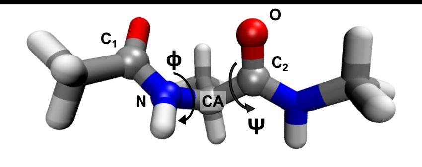
The 24th International Conference on Auditory Display (ICAD 2018)                           June 10 -15 2018, Michigan Technological University

data and maps these to sonic parameters. Previous sonifications                There is a question of the level of intervention that the soni-
of molecular simulation data seemed to have favoured PMSon                fication designer should take. If a dataset is rendered as directly
and auditory icons/earcons rather than model-based techniques.            as possible (i.e. converted to audio), then perhaps any audible fea-
This is likely because MD simulations already represent a physi-          tures present must be features of the data. But this rule may de-
cal model (see section 2.2) and adapting this dynamical system for        pend on the source and type of data (plus artifacts of the trans-
the purposes of model-based sonification is challenging.                  form). For example, a set of measurements of how temperature
     Rau et. al. [15] demonstrate a PMSon for interrogating fea-          changes over time might be treated differently to a non-local pa-
tures of a static molecule in the Megamol [16] visualization frame-       rameter that represents the overall instability of a system. In the
work. Their approach was to create audio representations of fea-          latter case, it may be necessary to map the data in a less direct way
tures that are known to be chemically interesting, such as the form-      to convey its provenance. Scaletti [25] categorises the directness
ing and breaking of hydrogen bonds. Sumo is a plug-in for the             of mappings through the idea of different orders: for 0th order, the
Python based molecular simulation environment PyMol [17].This             data is directly read as an audio waveform, for 1st order the data
project had the fairly broad aim of providing a general framework         is used to modulate a carrier signal. The approach presented here
for implementing various sonifications within PyMol. A relevant           uses many 1st order, one-to-many [26] mappings that attempt to
example application created parameterized earcons by mapping              create a certain perceptual effect related to the significance of a
the pairwise distances of all atoms of an amino acid onto the pa-         given feature. A problem that may be encountered with this ap-
rameters of a set of resonant filters. These were offset in both          proach is that it is atheroetical; the decisions made are based on
time and space according to their deviation from a reference amino        some subjective sound design process and the results often repre-
acid. Although no formal studies were undertaken, the designers           sent the designer’s sensibilities just as much as the underlying data
observed that it was possible to distinguish between them and thus        set [27]. The techniques used in this project are primarily param-
perceive conformational differences in the molecule [18]. Grond           eter mappings, which certainly do encounter some of the issues
et al show a technique for mapping structural information of sec-         raised above. Acknowledging these issues is important although
ondary RNA structures to sonic parameters with a view to aiding           addressing them all in detail is out of scope for this paper.
browsing and classification; however, there was no attempt to son-             This work extends the practice of molecular sonification by
ically render dynamical walks along free energy surfaces, which is        seeking an auditory display of how a molecule walks along a free
our focus here. [19]. Hermann describes some of the critical is-          energy landscape and its relation to fundamental dynamic pro-
sues that arise when designing a PMSon, observing that mappings           cesses of biomolecules, something that builds on our previous
are not necessarily transparent to a first time listener without some     work developing real-time sonification strategies for molecular dy-
kind of “code book” [20]. This point is reiterated by Wishart when        namics simulations ([28, 29, 30]). In these prior works, we sonified
describing the design of his piece, Supernova, which sonified as-         atomistic systems and events including atomic collisions, atomic
tronomical observations: “...there is no particular reason to use one     clustering, and vibrational spectra. This work focuses on the fea-
mapping rather than another. As a result, the sonic outcome would         tures of molecular systems. A simulation of the biomolecule Ala-
be entirely dependent on the mapping chosen.” [21].                       nine dipeptide (AD) is analysed using both hidden and observed
                                                                          Markov models to extract features of the underlying free energy
                                                                          landscape. These features are then mapped to sonic parameters
1.3. Molecular representation                                             to generate coupled visual and auditory display of structural and
Representational arbitrariness is a particularly interesting issue        dynamic information respectively.
when it comes to atomistic and molecular representations, owing                This paper is organized as follows: section 2 explains some
to the fact that they are too small to be experienced directly, ei-       of the underlying physical ideas and the modeling of biomolecular
ther visually or aurally. There is an inevitable degree of flexibil-      dynamics, section 3 explains our sonification strategy, some details
ity when designing representations of imperceptible phenomenon,           of the implementation are given in section 4, and our conclusions
which is evident in the range of available molecular visualisation        and outlook for further work are given in section 6. An example of
approaches, e.g., Pauling’s paper protein helices [22], Kendrew’s         the sonification described in this paper can be found at
metal, wood and plastic protein structures [23], and the increas-         https://vimeo.com/255391814.
ingly common digital ’ribbon renderings’.[24]. When it comes to
sonification, rendering conventions are far from established. De-          2. BIOMOLECULAR CONFORMATIONAL DYNAMICS
picting an atom as a sphere is, in some sense, an arbitrary deci-
sion, but makes some sense insofar as both are spatially delimited.       2.1. Free energy landscape
Attempting to define such a clearly delimited object in the audio
realm is not as straightforward, neither spatially nor composition-       Biomolecules such as proteins and nucleic acids are dynamic ob-
ally. It is difficult to assert what constitutes a single atomistic ob-   jects comprised of n atoms, each of which interacts with other
ject in a piece of sound design.                                          atoms in the same molecule and the cellular environment. A
     However, there are a wide range of “non-local” properties im-        molecular system has 3n degrees of freedom: each atom moves
portant in biomolecular science (e.g. potential energy, free energy,      in the x, y, and z direction. Typically biomolecules are comprised
electrostatic energy, temperature, conformational state member-           of thousands of atoms, leading to high-dimensional dynamics.
ship, etc.). Such properties are extremely difficult to visualize us-          At any given time, a molecule adopts a particular shape, or
ing conventional rendering strategies (and even if there were effec-      conformational state. Researchers are typically interested in un-
tive strategies, would lead to significant visual congestion) owing       derstanding the networks of conformational states that character-
to their non-locality. We believe that such properties are the most       ize a particular molecule. Networks of highly connected states in
interesting to explore in a sonification context: hence our focus on      which the system has a relatively long residence time are called
free energy in this work.                                                 metastable states. Of particular interest in many applications is
The 24th International Conference on Auditory Display (ICAD 2018) June 10 -15 2018, Michigan Technological University
understanding how long it takes a molecule to travel between dif-
ferent metastable states. Conformational states are of interest be-
cause they are directly linked to the molecule’s function, insight
[31] which has been verified extensively through experiments [32]
and computational studies [33, 34].
Any given conformational state has an associated free energy.
Highly probable conformations have a lower free energy than im-
probable conformations. Rises and falls in free energy as a func-
tion of molecular shape (atomic coordinates) define a free energy Figure 1: Atomic structure of Alanine dipeptide (AD). The cylin-
landscape, which is illustrated in further detail in what follows. ders represent chemical bonds and their intersections represent
atoms. Grey, blue, red and white colors are carbon, nitrogen, oxy-
2.2. Molecular dynamics simulation gen and hydrogen atoms respectively. The atoms involved in the
φ, ψ dihedral angles are labeled and highlighted as spheres. The φ
The output of MD simulations are a series of regularly timed snap- angle is formed from the intersection of the planes formed by the
shots (frames) of atomic configurations as the system evolves, atoms (C1 , N, CA) and (N, CA, C2 ). The ψ angle is formed from
called trajectories. An animated example trajectory can be viewed the planes formed by the atoms (N, CA, C2 ) and (CA, C2 , O).
at https://vimeo.com/255526473. With enough trajec-
tories it is possible to understand the probability that a molecule
occupies certain states, and develop a corresponding map of the a metastable state (A) given a particular observed state (a), i.e.
free energy landscape. The primary challenge in constructing such MA,a = P (Xt = A|xt = a). HMMs work well in describing
maps arises from the system’s high dimensionality. Researchers biomolecular dynamics in the regime where the underlying dy-
are therefore focussing on dimensionality reduction techniques namics are metastable. In other words the proportion of observed
for identifying only those coordinates (or combinations of coordi- states with membership probabilities intermediate between 0 and
nates) which take the system from one metastable state to another. 1 are small in comparison with the total number of observed states.
2.3. Markov Models 2.4. Alanine Dipeptide Model
Markov state models have found widespread use in recent years The “hello world” example of a biomolecule exhibiting metastable
as a dimensionality reduction technique to analyze the metastable dynamics is Alanine dipeptide (AD), as shown in figure 1. The
dynamics of biomolecules [35]. Their popularity stems from their metastable dynamics of AD are reasonably well described with
ability to produce predictive and easy to understand results as well reference to two dihedral angles made by atoms in the peptide
as their ability to parallelize the problem of resolving very long bonds [38], the φ and ψ angles, also shown figure 1. The free
timescale processes. Markov models transform a trajectory into a energy landscape of AD projected onto these two dimensions is
chain of n discrete states. These states are called observed states shown in figure 2A. The light yellow colour denotes free energy
(or sometimes microstates) and form the data from which both wells, i.e. regions with a low value of free energy which define
types of Markov model can be estimated. In general we refer to the metastable states. The lighter purple regions are those which
a chain as xt and a specific element by its position in the chain: are visited only briefly on the way to a metastable well, known as
x2 = 3 denotes that the second frame of the chain is in state 3. We transition regions. As the dihedral angles are periodic, conforma-
refer to the set of all possible discrete states as x. There are two re- tions with φ/ψ = 180◦ are equal to those with φ/ψ = −180◦ .
lated and widespread approaches: observed Markov state models This means that rather than a 2D plane, the free energy landscape
[36] and hidden Markov models [37]. This work uses both. actually resides on a torus, i.e. each edge of the chart should be
An observed Markov state model (or simply Markov state wrapped around to meet the opposite side. For the sake of simplic-
model, MSM) assumes the probability of transitioning to observed ity we show it here in the form in which it is typically rendered by
state b in a time τ given we are in state a, P (xt+τ = b|xt = a), practitioners in the field.
only depends on the states a and b and not on the states visited at For the purposes of this paper two models were created - an
times t − 1, t − 2, ..., 0. This property is known as the Markov observed MSM and a HMM. Details of the data and calculations
property and any chain that satisfies this is known as Markovian. used to generate the models can be found in section 4. The esti-
The dynamical information of the MSM is contained within a tran- mated transition matrix for the MSM results in 500 eigenvectors
sition matrix, T(τ ), whose elements are the conditional transition which describe the various relaxation modes of the dynamics. The
probabilities, i.e. T (τ )a,b = P (xt+τ = b|xt = a). first eigenvector q1 is equal to the stationary distribution, µ(x).
The primary problem with observed Markov state models is The next three eigenvectors are slow relaxation modes (q2,3,4 )
that they contain too much information: the observed states need which define population transfer between metastable states. The
clustering into a smaller number of metastable states in order to next five eigenvectors (q5−9 ) are fast relaxation modes which
make quantitative predictions about their dynamics. A hidden define population transfer within metastable states. Each relax-
Markov model (HMM) represents a sort of fuzzy clustering of the ation mode has an associated timescale (the corresponding eigen-
observed states into a set of metastable states (or hidden states, value). The remaining eigenvectors were discarded as the associ-
X), i.e. instead of describing a particular conformation (observed ated timescales for these modes was faster than the time resolution
state) as unambiguously belonging to a metastable state, a prob- of the data used to estimate the model and so were not considered
ability of membership is given. A HMM consists of a transi- statistically robust. The HMM was estimated by assuming four
tion matrix for the metastable states and a membership matrix metastable states. The results are shown in figure 2. Figure 2D
M whose elements are the conditional probability of being in shows the metastable state transition matrix, T. Each circle repre-The 24th International Conference on Auditory Display (ICAD 2018) June 10 -15 2018, Michigan Technological University
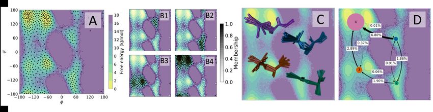
Figure 2: The hidden Markov model for AD. A: The free energy landscape of AD projected onto the peptide φ and ψ dihedral angles.
The lighter the colour the lower the free energy and hence the more stable those atomic configurations. The yellow regions define four
metastable basins centered on coordinates (60◦ , 60◦ ), (60◦ , −120◦ ), (−120◦ , −60◦ ), (−120◦ , 120◦ ). The purple regions are not visited
during the simulations used as input for the model. The black circles are the centers of 500 observed states for both the observed and
hidden Markov models. Each frame of the trajectory is assigned to the nearest observed state.B1-4: Each panel represents rows 1 - 4 of the
membership matrix. Each circle represents an observed state coloured according to its membership probability to each metastable state. C:
Ten sampled conformations of each metastable state of AD overlaid over the center of their free energy well. The hydrogen atoms have
been removed for clarity. D: The transition matrix and stationary distribution of metastable states. Each circle represents a metastable state
with the area of each circle proportional to the stationary distribution. The arrows between each state show possible transitions with the
width proportional to the conditional transition probability (also shown in the white boxes on each arrow).
sents a metastable state with the area of the circle proportional to Type Scope Parameter Layer
its stationary distribution, µ(X1,...,4 ). The arrows show the con- Dynamic Intra Free Energy F (a) B
Fast Mode [qi ]a
ditional probability of transitioning to each state. For example, the C
probability of transitioning from state 1 to state 4 is 6.79%. State 4 Inter Shannon Entropy Ha A
is by far the most stable, followed by 3, 2 and then 1. As there are Membership
no transition regions between state 1 and 3 and between 2 and 4, probability [M]a A
the probability of transitions between these pairs of states is zero. Static Well min U L[h] A
Figure 2C shows an overlay of ten characteristic structures for each Well max U B[h] A
metastable state, overlaid over their respective free energy wells. Histogram area A[h] A
Figures 2B1-4 show the rows of the membership matrix. Each cir-
cle represents one of the observed states, coloured according to the Table 1: Simulation features exposed via OSC. Type refers to
membership probability to each metastable state. The partitioning whether the features are fixed at time 0 (static) or change at each
of the basins is clearly shown by the regions of black circles (high trajectory frame (dynamic). Scope refers to whether the features
probability of metastable membership) vs. white circles (low prob- relate to transitions between states (inter) or within a state (intra).
ability of metastable membership).
3. SONIFICATION
molecule and do not change after they are initialised at time 0. Dy-
namic features are those derived from each frame (i.e. from each
The sonification is designed to convey features of the free energy observed state) of the example trajectory as well as the model fea-
landscape concurrently alongside visual display of structural infor- tures. As well as categorizing the features as static or dynamic, a
mation, i.e., a molecular animation from an example trajectory. It further distinction is drawn between those that relate to changes
therefore requires three objects: a model of AD dynamics, an ex- within the current metastable state (intrastate) and those that per-
ample trajectory and an animation of the example trajectory. In this tain to changes between the metastable states (interstate). Table 1
work the data used to estimate the model of AD (the input trajec- summarizes these two categorizations. This second classification
tories) are different to the example trajectory although in principle is useful because it draws the distinction between features based
trajectories from the input data could be used as example trajecto- on characteristics of the physical dynamics rather than how they
ries. The following section provides a description of the features were generated. The interstate features represent the most phys-
derived from the data followed by a description of the components ically important characteristics of the dynamics and free energy
of the sonification and how features of the data are mapped to syn- landscape and so form the core of the mapping strategy.
thesis parameters.
Firstly, we discuss static features: these are derived from the
shape of the free energy wells associated with each metastable
3.1. Free Energy Landscape Features state. Each part of the free energy landscape is assigned a prob-
ability of membership to a metastable state so the limits of each
The features of the data are split into two categories: static and well are not well defined. In order to overcome this problem each
dynamic. Static features are derived from the properties of the AD observed state is assigned to the metastable state for which it hasThe 24th International Conference on Auditory Display (ICAD 2018) June 10 -15 2018, Michigan Technological University
the highest probability of membership. The three static features for 1
each metastable state, U B[h], LB[h], A[h] are interstate features. State 1
They are principally related to two physical characteristics: the 0
relative stability and conformational flexibility of each metastable 1
state. The focus of the mapping strategy is to find a way to de- State 2
scribe them aurally. The free energy for each observed state a, 0
F (a) = −kT ln(µ([x]a )) was calculated and scaled to lie in the 1
range (0, 1). Here k refers to the Boltzmann constant and T to State 3
0
the temperature. The static features for each metastable state were 1
derived from a histogram of the free energies of observed states
assigned to that metastable state. We denote the histogram for
State 4
metastable state A as hA (F ) (or h in general). The properties we
0
1
Free Shannon
Entropy
derive from h(F ) are (1) its upper bound, U B[h], (2) its lower
R1
bound LB[h] (3) its area A[h] = 0 dF h(F ). The histograms
for states 1 (blue) and 4 (pink) are shown in figure 5. The model 0
has four metastable states meaning there are 4 × 3 = 12 static 1
Mode 5 energy
features. The upper and lower bounds are related to the free en-
ergy well minima and maxima for each metastable state. The area
of the histograms is proportional to the overall volume of the free 0
energy well. 1
Secondly, we discuss dynamic features: these change with 0
each observed state in the example trajectory. For each ob-
served state they are: (1) its probability of membership to each 1
of the four metastable states, (2) the Shannon entropy of its 80.00 80.02 80.04 80.06 80.08 80.10
metastable state assignments (3) its absolute free energy, (4) its Time (ns)
projection into the five fast relaxation modes. For each observed
state there are 4 + 1 + 1 + 5 = 11 dynamic features. The Figure 3: The dynamic features of the model. Each panel shows
membership probability describes the probability that a given ob- how a model features varies over 0.1ns (100 frames) of the ex-
served state can be assigned to a given metastable state. For ob- ample trajectory. State 1-4 show the membership probability of
served state a there are four membership probabilities given by each frame’s observed state to each metastable state. The values
([M]1,a , [M]2,a , [M]3,a , [M]4,a ). The information or Shannon in each frame across all four panels sum to 1. Shannon entropy
entropy is a measure of the degree of certainty with which the measures the uncertainty of the assignment of each observed state
assignment of an observed state to a particular metastable state to the metastable states. High entropy indicates an observed state
can be made. The Shannon P entropy for an observed state a, Ha could be considered to belong to more than one metastable state.
is given by Ha = − 4i=1 [M]i,a ln([M]i,a ). Ha = 0 in- Free energy is the free energy of each observed state, the lower the
dicates the observed state is definitely in one metastable state. free energy the more stable the state. Mode 5 is the first fast re-
Ha = ln(4) ≈ 1.4 indicates it is equally likely to be in any of laxation mode which redistributes population within a metastable
the four metastable states. The free energy of observed state a, state. The other four fast modes are not shown.
F (a) measures the observed state’s global stability. These were
the same free energies used in the calculation of the static features
in section 3.1. The projection of observed state a onto the i’th fast
relaxation modes is given by [qi ]a . Large oscillations in a pro- 2 Synthesis: Created using a subtractive, polyphonic synthesiser
jection indicate that the system is relaxing along that mode. The with noise as a source signal. The basic signal flow of a sin-
values of these projections were scaled to lie in the range (−1, 1). gle voice is shown in Figure 4 . The main parameters are the
Figure 3 shows the dynamic features for a section of an example Q value of the resonant filter, the depth and rate of frequency
trajectory. modulations for each voice and the amplitude of each voice.
3 Mapping: Each metastable state is characterised by a set of
notes referred to as a note cluster. This design arises from the
3.2. Sonification Layers
desire to represent metastable state transitions by tonal group-
As the molecule traverses different regions of the free energy land- ings, a musical device that non-trained listeners should be able
scape the sonification conveys information about its properties to perceive. The maximum note range is predefined to three oc-
with the following layers in the audio stream: (A) a continuous taves. The relative values of A[h] for each metastable state de-
pad sound representing membership of different metastable states fines the number of notes in its corresponding note cluster, these
and their properties, (B) a pulse sound representing the stability of notes are then evenly distributed between the lowest and highest
the system and (C) a set of synthesized tones that represent how notes. The values of LB[h] and U B[h] define the lowest and
the system is changing within each metastable state. highest notes of each cluster respectively. This is shown in fig-
The Pad Sound (A) was constructed as follows: ure 5 for metastable states 1 and 4. State 4 (pink) has a smaller
range, but a larger area resulting in a dense, tightly spaced note
1 Representation: The pad sound represents features of the cluster at the lower extent of the note range. State 1 (blue) has a
well in the free energy landscape corresponding to the current large range but small area resulting in a more sparse note clus-
metastable state assignment. ter. State 4 has its lower bound below that of state 1 and soThe 24th International Conference on Auditory Display (ICAD 2018) June 10 -15 2018, Michigan Technological University
Entropy
f
Normalise
(0-1)
1
a
a-b
b
!- 1
Frequency
Uniform Noise 30 Hz
f q f
Out
Figure 4: Single synthesis voice as used for each note of a
metastable state note cluster. The set of multiple instances (one Figure 5: The mapping of static properties of the metastable states
per note) form the pad sound. The inputs are the frequency of each to note clusters. Each of the observed states was first assigned to
note in the note cluster and the entropy. The note cluster is deter- exactly one metastable state. The bottom chart shows the distribu-
mined by the membership probability values at the current frame. tion of free energies of observed states which have been assigned
to the metastable states 1 (blue) and 4 (pink). States 2 and 3 are not
shown for clarity. The coloured notes of the keyboard are the note
the lowest note of the cluster is below that of state 1. An ac- clusters used to represent the metastable states. The relative upper
cepted limitation of this mapping is that it does not attempt to and lower bounds of the distributions determine the highest and
classify the clusters in terms of their harmonic relationships. In- lowest notes in the cluster (as shown by the vertical connectors).
stead, it deals with them as distributions of notes within a range, The relative area of each distribution determines the number of
with a given extent and density. It may be possible to create a notes in the note cluster. The ratio of the areas of state 4’s distribu-
hierarchy of tonal groupings from which to choose but this is tion to state 1’s distribution is approximately 3:1. This determines
highly genre specific. This is an outstanding issue in that listen- the 9:3 ratio of the number of notes in each note cluster.
ers may interpret the harmonic relationship of two note clusters
as significant when this is not intended as part of the mapping
(e.g. stacked whole tones vs. stacked fourths). The membership 2 Synthesis: Generated by sweeping the frequency of a sine
probabilities (M) control the choice of note cluster by linearly wave from approximately 130Hz to 20Hz over a short period
interpolating between the values defined by the static parame- (100-550ms) and passing it through a hard clipping function
ters of each state. This means that if [M]1,a = 1 then the clus- and stereo delay line. The relevant parameters are the rate at
ter defined by the static properties of metastable state 1 will be which the sweep is triggered, the length of time the sweep takes,
used. In the case that [M]1,a = [M]2,a = 0.5 then the lowest the amount of drive in the hard clipping function and the amount
and highest notes will lie halfway between those defined by the of feedback in the delay path.
static parameters of state 1 and 2. Large values of the Shannon 3 Mapping: The synthesis parameters are mapped to the absolute
entropy (H) represent observed states which could be assigned free energy F (xt ). The variable is inverted and filtered logarith-
to more than one metastable state, physically this means they mically. The filter settings are slightly different for each synthe-
are in transition regions between two metastable states. H is sis parameter but, in general terms, act to allow fast increases in
mapped to the width and rate of frequency modulations of the its values and slow decreases to ensure the temporal alignment
voices for the note clusters as well as the bandwidth of the filter between visual and sonic representations. The (F (xt )) of each
such that it tends toward noise for higher values of H. This is a observed state measures its stability relative to the global free
one-to-many mapping that is designed to create a perceptual ef- energy minimum. This feature allows the sonification to draw
fect of instability. H tends to remain at 0 with occasional spikes a distinction between an observed state being globally unstable
as the system transitions. This is shown in figure 3 where there and yet part of a relatively stable metastable state (or vice versa).
are spikes between 80.05 and 80.06 nanoseconds as transitions Within-Metastable State Tones (C) were constructed as follows:
occur between all four states. These spikes, although fleeting,
1 Representation: The extent to which the system is relaxing
are important features. To emphasise transitions an asymmet-
along one of the fast modes. This gives an impression of high
ric smoothing function is employed such that H values increase
frequency movements of the molecule that are not represented
quickly but decrease slowly.
by the membership probabilities.
The Pulse sound (B) was constructed as follows: 2 Synthesis: The fast mode projections are oscillatory signals be-
1 Representation: The overall stability of the current observed tween -1 and 1 and are exported as PCM wav files (a 0th order
state in relation to the global minimum. The pulse sound is de- mapping in Scaletti’s terminology [25]). At the 20Hz frame-
signed to underpin the entire sonification. The rationale here is rate being used for the animation the oscillations are subsonic.
that a rhythmic kick drum sound is commonly used as a rhyth- Scanned synthesis is used in order to render the content as au-
mic marker upon which all other elements are constructed. This dible [39]. The relevant parameter is the audio file that is used
mirrors the way in which the free energy landscape underpins as the wavetable to be scanned. Other parameters that affect the
the dynamics of the physical system. sound are the window size and the scanning frequency.The 24th International Conference on Auditory Display (ICAD 2018) June 10 -15 2018, Michigan Technological University
3 Mapping: Scanned synthesis was developed to allow for the di- the current observed state. The pulse/kick layer (B) is correlated
rect manipulation of synthesis timbre using a physical model to the absolute free energy; at 00:10, the current metastable state
and represents an extension of wavetable synthesis. In this case has a lower absolute free energy and the rate, level of distortion
it allows for a rolling window of the audio buffer to be scanned and delay feedback are increased resulting in the sound becoming
at a given frequency, with the effect that increased frequency more prominent. The layer representing the fast relaxation modes
and amplitude of oscillation in the window results in a brighter (C) can be heard as the metallic, buzzing sounds panned across
timbre. These can be heard panned from hard left (mode q5 ) to the sound-field. The scanned synthesis method means that ampli-
hard right (mode q9 ). The scanning frequency is defined by the tude and frequency of activity in the data is correlated to density of
lowest note of the set of note clusters (effectively the root of the spectra and amplitude of the synthesiser. So an increase in bright-
most stable state). ness of this sound on the left of the sound-field indicates that the
molecule is relaxing along the first of the five modes used.
4. IMPLEMENTATION
6. CONCLUSIONS AND FUTURE WORK
The simulation data was taken from a publicly available repository
which accompanies the paper [38] found at https://simtk. We have presented a strategy for representing features of the dy-
org/projects/alanine-dipeptide/. A full explanation namics and the free energy landscape of Alanine Dipetide with
of the methods used to generate the data are given in the paper. All sound. This auditory display can be used in tandem with visual dis-
modelling was done using the Python 3.5 programming language, play techniques to help build an understanding of how the physical
the Markov models were generated by PyEMMA 2.4 [40]. Both structure of AD relates to the underlying free energy landscape and
the HMM and MSM used the same set of 500 observed states and the resulting dynamic processes. Future user studies with domain
each were estimated with a lag time of τ = 1.0ps. The HMM experts will allow an assessment of the efficacy of the sonification;
was estimated by specifying four metastable states. This number a sketch for this would entail participants viewing an animation of
was chosen so that the approximation of metastability was most a simulation trajectory with and without the various layers of the
accurate at the lag time used. The molecular animations were gen- sonification to assess if and how they show an increased apprecia-
erated using VMD [24]. A 500ns long example trajectory was used tion of the free energy dynamics. In the future we hope to extend
in the sonification. This was generated from the HMM, rather than this implementation to allow a degree of interactivity in manipu-
using an input trajectory as they were all of insufficient length to lating the example trajectory. Initially, this would take the form
sample each metastable state regularly. While this trajectory does of allowing the user to manipulate the playback position, speed
not strictly obey the original equations of motion used to gener- and loop points of the trajectory. This would allow them to focus
ate the input data it reproduces all the modelled features (transi- on regions of interest in the dynamics. In the long term, allow-
tion probabilities, relaxation time-scales, stationary distribution) ing the user to manipulate the example trajectory using interactive
and so is indistinguishable from a trajectory generated using the molecular dynamics (for example, NanoSimbox [41]) and hear the
original equations of motion. A Python script, using the package resultant sonic effects is an exciting prospect and opens up the pos-
OSC 1.6.4, was used to create a client which sent the static and sibility of using the system as an instrument for musical expression
dynamic parameters as messages to the audio processing software. as well as data exploration.
The messages were sent using the OSC protocol. The dynamic
parameters were sent at a rate of 20 trajectory frames per second 7. ACKNOWLEDGMENT
(corresponding to a ratio of 20ps to 1s simulation to physical time).
The audio processing was implemented in Max/MSP. David Glowacki acknowledges funding from the Royal Society
Everything required to reproduce this work (except (UF120381) and the Leverhulme Trust. Robert Arbon is funded
the input data which can be downloaded separately) can by the Royal Society (RG130510). Alex Jones is supported by a
be found at https://osf.io/rzp3k/?view_only= studentship from the EPSRC and Interactive Scientific Ltd. Lars
b5802dfce6da4dd59dfb6b406ae033f0. Bratholm acknowledges EPSRC grant EP/P021123/1.
5. EXAMPLE SONIFICATION 8. REFERENCES
The example provided (link in sec. 1) shows an animation of an [1] R. P. Feynman, et al., The Feynman lectures on physics.
excerpt of trajectory data for Alanine Dipeptide accompanied by Addison-Wesley, 1963.
our sonification. This section provides a description of the audi- [2] M. Hashimoto, et al., “Role of Protein Aggregation
ble features and how they relate to the mapping strategy. The pad in Mitochondrial Dysfunction and Neurodegeneration in
layer (A) provides information about the structure of the free en- Alzheimer’s and Parkinson’s Diseases,” NeuroMolecular
ergy landscape for the configuration at a given frame; it can be Medicine, vol. 4, pp. 21–35, 2003.
heard ramping between the note clusters defined by the static fea-
[3] P. Singh, et al., “Linking Protein Motion to Enzyme Cataly-
tures of the four metastable states. It stays primarily in state 4,
sis,” Molecules, vol. 20, no. 1, pp. 1192–1209, 2015.
as this is the most stable. At 00:13 the animation shows a sig-
nificant change in the dihedral angles; this is linked to a change [4] S. A. Adcock and J. A. McCammon, “Molecular dynamics:
in the metastable state and a shift to a different well on the free Survey of methods for simulating the activity of proteins,”
energy landscape, which is depicted by the change in note clus- Chemical Reviews, vol. 106, no. 5, pp. 1589–1615, 2006.
ter of the pad sound. The noise/wind effect that can be heard at [5] D. Antoniou, et al., “Computational and Theoretical Meth-
00:10 is caused by an increase in the Shannon entropy and gives ods to Explore the Relation between Enzyme Dynamics and
an indication that there is some uncertainty in the assignment of Catalysis,” Chemical Reviews, vol. 106, no. 8, p. 3170, 2006.The 24th International Conference on Auditory Display (ICAD 2018) June 10 -15 2018, Michigan Technological University
[6] M. W. van der Kamp, et al., “Biomolecular simulation and [24] W. Humphrey, et al., “VMD – Visual Molecular Dynamics,”
modelling: status, progress and prospects,” J. Royal Society Journal of Molecular Graphics, vol. 14, pp. 33–38, 1996.
Interface, vol. 5, no. Suppl 3, p. 173, 2008. [25] C. Scaletti, “Sound synthesis algorithms for auditory data
[7] J. E. Stone, et al., “Gpu-accelerated molecular modeling representations,” in Auditory Display: Sonification, Audifi-
coming of age,” J. Molecular Graphics and Modelling, cation, And Auditory Interfaces, G. Kramer, Ed. Reading:
vol. 29, no. 2, p. 116, 2010. Addison-Wesley, 1994.
[8] P. Eastman, et al., “Openmm 4: A reusable, extensible, hard- [26] A. Hunt, et al., “The Importance of Parameter Mapping in
ware independent library for high performance molecular Electronic Instrument Design,” Journal of New Music Re-
simulation,” J. Chemical Theory and Computation, vol. 9, search, vol. 32, no. 4, pp. 429–440, 2003.
no. 1, p. 461, 2013. [27] E. Murphy, et al., “A Semiotic Approach to the Design of
Non-speech Sounds,” in Haptic and Audio Interaction De-
[9] D. Case, et al., “Amber 2017,” University of California, San
sign, D. McGookin and S. Brewster, Eds. Berlin, Heidel-
Francisco, 2017.
berg: Springer Berlin Heidelberg, 2006, pp. 121–132.
[10] M. Álvarez-Moreno, et al., “Managing the computational [28] D. R. Glowacki, et al., “A gpu-accelerated immersive audio-
chemistry big data problem: The iochem-bd platform,” J. visual framework for interaction with molecular dynamics
Chemical Information and Modeling, vol. 55, p. 95, 2015. using consumer depth sensors,” Faraday Discuss., vol. 169,
[11] B. J. Alder and T. E. Wainwright, “Studies in molecular dy- pp. 63–87, 2014.
namics. i. general method,” J. Chemical Physics, vol. 31, [29] T. Mitchell, et al., “danceroom spectroscopy: At the fron-
no. 2, p. 459, 1959. tiers of physics, performance, interactive art and technology.”
[12] P. W. Atkins and J. de Paula., Atkins’ physical chemistry, Leonardo, vol. 49, no. 2, pp. 138–147, 2016.
10th ed., 2014. [30] D. Glowacki, “Sculpting molecular dynamics in real-time us-
[13] G. Prez-Hernndez, et al., “markovmodel/molPX: More ing human energy fields,” in Molecular Aesthetics, P. Weibel
PyEMMA integration through handling of TICA objects,” and L. Fruk, Eds. Cambridge, MA: The MIT Press, 2013,
Mar. 2017. [Online]. Available: https://doi.org/10.5281/ pp. 248–257.
zenodo.437707 [31] H. Frauenfelder, et al., “The energy landscapes and motions
[14] T. Hermann and H. Ritter, “Listen to your Data: Model- of proteins,” Science, vol. 254, no. 5038, p. 1598, 1991.
Based Sonification for Data Analysis,” in Advances in in- [32] Y. Santoso, et al., “Conformational transitions in dna poly-
telligent computing and multimedia systems. Inst. for Ad- merase i revealed by single-molecule fret,” P. National
vanced Studies in System research and cybernetics, 1999, pp. Academy of Sciences, vol. 107, no. 2, p. 715, 2010.
189–194. [33] D. Wales, Energy Landscapes: Applications to Clusters,
[15] B. Rau, et al., “Enhancing visualization of molecular sim- Biomolecules and Glasses, ser. Cambridge Molecular Sci-
ulations using sonification,” in 1st International Workshop ence. Cambridge University Press, 2004.
on Virtual and Augmented Reality for Molecular Science. [34] N.-V. Buchete and G. Hummer, “Coarse master equations for
IEEE, March 2016, pp. 25–30. peptide folding dynamics,” J. Physical Chemistry B, vol. 112,
no. 19, p. 6057, 2008, pMID: 18232681.
[16] S. Grottel, et al., “MegaMol-A prototyping framework for
particle-based visualization,” IEEE Transactions on Visual- [35] J. D. Chodera and F. Noé, “Markov state models of
ization and Graphics, vol. 21, pp. 201–214, February 2015. biomolecular conformational dynamics,” Current Opinion in
Structural Biology, vol. 25, pp. 135 – 144, 2014.
[17] “Pymol,” 2017. [Online]. Available: https://pymol.org/2/
[36] J.-H. Prinz, et al., “Markov models of molecular kinetics:
[18] F. Grond and F. Dall Antonia, “Sumo. A Sonification Utility Generation and validation,” The Journal of chemical physics,
for Molecules,” in Proceedings of ICAD 2008, no. 14. In- vol. 134, no. 17, p. 174105, 2011.
ternational Community for Auditory Display, 2008, pp. 1–7.
[37] F. Noé, et al., “Projected and hidden markov models
[19] F. Grond, et al., “Browsing RNA Structures by Interactive for calculating kinetics and metastable states of complex
Sonification,” in ISon, 3rd Interactive Sonification Workshop, molecules,” The Journal of chemical physics, vol. 139,
Stockholm, 2010, pp. 11–16. no. 18, p. 184114, 2013.
[20] T. Hermann, et al., “Sonification of markov chain monte [38] J. D. Chodera, et al., “Automatic discovery of metastable
carlo simulations,” in ICAD 2001. Espoo, Finland: Georgia states for the construction of markov models of macromolec-
Institute of Technology, 2001, pp. 208–216. ular conformational dynamics,” J. Chemical Physics, vol.
126, no. 15, p. 155101, 2007.
[21] T. Wishart, “From Sound Morphing to the Synthesis of
Starlight. Musical experiences with the Phase Vocoder over [39] B. Verplank and R. Shaw, “Scanned Synthesis,” The Journal
25 years,” Musica/Tecnologia, vol. 7, 2013. of the Acoustical Society of America, vol. 109, no. 5, 2001.
[22] L. Pauling, et al., “The structure of proteins: Two hydrogen- [40] M. K. Scherer, et al., “PyEMMA 2: A Software Package for
bonded helical configurations of the polypeptide chain,” P. Estimation, Validation, & Analysis of Markov Models,” J.
National Academy of Sciences, vol. 37, no. 4, p. 205, 1951. Chemical Theory & Computation, vol. 11, p. 5525, 2015.
[41] M. O. Connor, et al., “Sampling molecular conformations
[23] J. C. Kendrew, et al., “A three-dimensional model of the
and dynamics in a multi-user virtual reality framework,”
myoglobin molecule obtained by x-ray analysis,” Nature,
ArXiv e-prints, Jan. 2018, ArXiv:1801.02884.
vol. 181, p. 662, 03 1958.You can also read